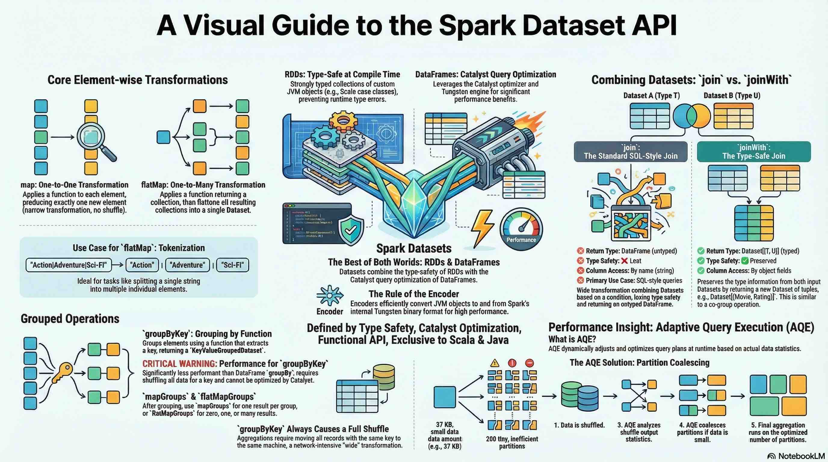
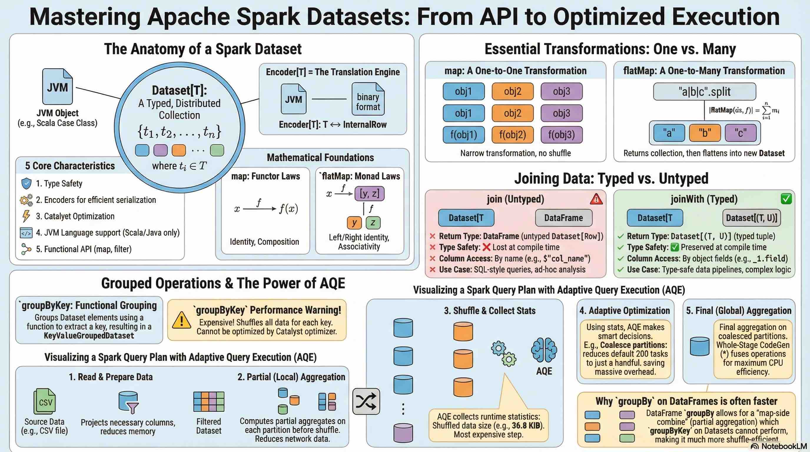
Spark Dataset APIs
- Introduction
- Dataset Transformations
- Grouped Operations
Introduction
What are Datasets?
Apache Spark Datasets are the foundational type in Spark’s Structured APIs, providing a type-safe, distributed collection of strongly typed JVM objects. While DataFrames are Datasets of type Row, Datasets allow you to define custom domain-specific objects that each row will consist of, combining the benefits of RDDs (type safety, custom objects) with the optimizations of DataFrames (Catalyst optimizer, Tungsten execution).
Key Characteristics:
- Type Safety: Compile-time type checking prevents runtime type errors
- Encoders: Special serialization mechanism that maps domain-specific types to Spark’s internal binary format
- Catalyst Optimization: Benefits from Spark SQL’s query optimizer
- JVM Language Feature: Available only in Scala and Java (not Python or R)
- Functional API: Supports functional transformations like
map,filter,flatMap
Dataset[T]: A distributed collection of data elements of type T, where T is a domain-specific class (case class in Scala, JavaBean in Java) that Spark can encode and optimize.
Translation: A Dataset of type T is a collection of n elements, where each element belongs to type T.
Encoder[T]: A mechanism that converts between JVM objects of type T and Spark SQL’s internal binary format (InternalRow).
Translation: An Encoder for type T provides bidirectional conversion between objects of type T and Spark’s internal row representation.
Dataset Movie Lens
Let’s examine the MovieLens dataset: recommended for education and development for simplicity.
---
config:
  look: neo
  theme: default
---
erDiagram
    Movies ||--o{ Ratings : "receives"
    Movies ||--o{ Tags : "has"
    Movies ||--|| Links : "references"

    Movies {
        int movieId PK "Primary Key"
        string title "Movie title with year"
        string genres "Pipe-separated genres"
    }

    Ratings {
        int userId FK "Foreign Key to User"
        int movieId FK "Foreign Key to Movie"
        float rating "Rating value (0.5-5.0)"
        long timestamp "Unix timestamp"
    }

    Tags {
        int userId FK "Foreign Key to User"
        int movieId FK "Foreign Key to Movie"
        string tag "User-generated tag"
        long timestamp "Unix timestamp"
    }

    Links {
        int movieId PK "Primary Key"
        int movieId FK "Foreign Key to Movie"
        string imdbId "IMDB identifier"
        string tmdbId "TMDB identifier"
    }
Entities and Attributes
- Movies (9,742 movies)
movieId(Primary Key)title(includes release year)genres(pipe-separated list)
- Ratings (100,836 ratings)
userId(Foreign Key)movieId(Foreign Key)rating(0.5 to 5.0 stars)timestamp(Unix timestamp)
- Tags (3,683 tags)
userId(Foreign Key)movieId(Foreign Key)tag(user-generated metadata)timestamp(Unix timestamp)
- Links (9,742 links)
movieId(Primary Key & Foreign Key)imdbId(IMDB identifier)tmdbId(The Movie Database identifier)
Relationships
- Movies ↔ Ratings: One-to-Many (a movie can have multiple ratings)
- Movies ↔ Tags: One-to-Many (a movie can have multiple tags)
- Movies ↔ Links: One-to-One (each movie has one set of external links)
Let’s define the Case class
case class Movie(
  movieId: Int,
  title: String,
  genres: String
)
defined class Movie
Create a DataSet using the above Case class:
// Read CSV and convert to Dataset
val moviesDS = spark.read
  .option("header", "true")
  .option("inferSchema", "true")
  .csv("ml-latest-small/movies.csv")
  .as[Movie]

// Example queries
moviesDS.show(4)
+-------+--------------------+--------------------+
|movieId|               title|              genres|
+-------+--------------------+--------------------+
|      1|    Toy Story (1995)|Adventure|Animati...|
|      2|      Jumanji (1995)|Adventure|Childre...|
|      3|Grumpier Old Men ...|      Comedy|Romance|
|      4|Waiting to Exhale...|Comedy|Drama|Romance|
+-------+--------------------+--------------------+
only showing top 4 rows


moviesDS: Dataset[Movie] = [movieId: int, title: string ... 1 more field]
Key Points:
- Case classes must be serializable
- All fields should have Spark-compatible types
- The
.as[T]method performs the conversion from DataFrame to Dataset
Understanding Encoders
Encoders are a critical component of the Dataset API. They provide:
- : Convert JVM objects to Spark’s internal Tungsten binary format
- : Automatically infer schema from case class structure
- : Enable whole-stage code generation for better performance
import org.apache.spark.sql.Dataset
// for primitive types
val intDS : Dataset[Int] = Seq(1,2,3).toDS()
import org.apache.spark.sql.Dataset
intDS: Dataset[Int] = [value: int]
val tupleDS: Dataset[(String, Int)] = Seq(("a",1), ("b", 2)).toDS()
tupleDS: Dataset[(String, Int)] = [_1: string, _2: int]
Using Case classes:
case class Dog(name: String, age: Int)
defined class Dog
val dogsDS: Dataset[Dog] = Seq(Dog("Liela",3), Dog("Tommy", 5)).toDS()
dogsDS: Dataset[Dog] = [name: string, age: int]
dogsDS.show()
+-----+---+
| name|age|
+-----+---+
|Liela|  3|
|Tommy|  5|
+-----+---+
Dataset Transformations
map Transformation
The map transformation applies a function to each element in the Dataset, producing a new Dataset with transformed elements. It’s a narrow transformation (no shuffle required) and maintains a one-to-one relationship between input and output elements.
Signature:
def map[U](func: T => U)(implicit encoder: Encoder[U]): Dataset[U]
f: function
For example, to extract the movie title:
moviesDS.map(m => m.title).show(3, truncate=false)
+-----------------------+
|value                  |
+-----------------------+
|Toy Story (1995)       |
|Jumanji (1995)         |
|Grumpier Old Men (1995)|
+-----------------------+
only showing top 3 rows
def extractMovieInfoFun(movie: Movie): (String, String) = (movie.title, movie.genres)
moviesDS.map(extractMovieInfoFun)
defined function extractMovieInfoFun
res11_1: Dataset[(String, String)] = [_1: string, _2: string]
As shown above, you can create a function.
Or you can create a anonymous function as follows:
val extractMovieInfoAnonymousFun: Movie => (String, String) = movie => (movie.title, movie.genres)
moviesDS.map(extractMovieInfoAnonymousFun)
extractMovieInfoAnonymousFun: Movie => (String, String) = ammonite.$sess.cmd12$Helper$$Lambda$6705/0x00007f74dd5ef838@1c5f48b8
res12_1: Dataset[(String, String)] = [_1: string, _2: string]
Above can be directly written in the map function:
moviesDS.map(movie => (movie.title, movie.genres))
res13: Dataset[(String, String)] = [_1: string, _2: string]
flatMap Transformation
The flatMap transformation applies a function to each element and flattens the results. Each input element can produce zero, one, or multiple output elements. This is essential for transformations like tokenization, exploding nested structures, or filtering with expansion.
Signature:
def flatMap[U](func: T => TraversableOnce[U])(implicit encoder: Encoder[U]): Dataset[U]
Translation: Given a function that transforms each element of type T into a collection of type U, flatten all collections into a single Dataset of type U.
- Monad Operation: flatMap enables chaining transformations that produce collections
- One-to-Many Mapping: Input orders (3) produce output items (6)
- Demonstrates nested iteration flattening
For a Dataset with $n$ elements, where each element produces $m_i$ results:
\[|\text{flatMap}(ds, f)| = \sum_{i=1}^{n} m_i\]Translation: The size of the flatMapped Dataset equals the sum of results from each element’s transformation.
case class MovieGenres (id: Int, genres: String)
defined class MovieGenres
val genres = moviesDS.map { movie =>
    MovieGenres(movie.movieId, movie.genres)
}
genres: Dataset[MovieGenres] = [id: int, genres: string]
genres.show(3, truncate=false)
+---+-------------------------------------------+
|id |genres                                     |
+---+-------------------------------------------+
|1  |Adventure|Animation|Children|Comedy|Fantasy|
|2  |Adventure|Children|Fantasy                 |
|3  |Comedy|Romance                             |
+---+-------------------------------------------+
only showing top 3 rows
val genresDS = genres.flatMap(m => m.genres.split("\\|"))
genresDS.show(5)
+---------+
|    value|
+---------+
|Adventure|
|Animation|
| Children|
|   Comedy|
|  Fantasy|
+---------+
only showing top 5 rows


genresDS: Dataset[String] = [value: string]
The
split()method takes a regex pattern, and|is a special character in regex meaning “OR”. Sosplit("|")doesn’t work as expected. Instead, usesplit("\\|")for split.
Complex Example: Nested Structure Explosion
case class GenreOccurences(id: Int, words: Seq[String], occurrences: Seq[Int])
// companion object for the above case class
object GenreOccurences {
  def fromMovie(movie: Movie): GenreOccurences = {
    val id = movie.movieId
    val text = movie.genres

    // Extract words
    val words = text.split("\\|").toSeq

    // Count occurrences of each word
    val wordCounts = words.groupBy(identity).view.mapValues(_.size).toMap
    val occurrences = words.map(word => wordCounts(word))

    GenreOccurences(id, words, occurrences)
  }
}
defined class GenreOccurences
defined object GenreOccurences
val genreOccurencesDS: Dataset[GenreOccurences] = moviesDS.map(GenreOccurences.fromMovie)
genreOccurencesDS: Dataset[GenreOccurences] = [id: int, words: array<string> ... 1 more field]
genreOccurencesDS.show(3, truncate=false)
+---+-------------------------------------------------+---------------+
|id |words                                            |occurrences    |
+---+-------------------------------------------------+---------------+
|1  |[Adventure, Animation, Children, Comedy, Fantasy]|[1, 1, 1, 1, 1]|
|2  |[Adventure, Children, Fantasy]                   |[1, 1, 1]      |
|3  |[Comedy, Romance]                                |[1, 1]         |
+---+-------------------------------------------------+---------------+
only showing top 3 rows
genreOccurencesDS.flatMap { genreOccurence =>
    genreOccurence.words.zip(genreOccurence.occurrences).map { case (word, numOccured) =>
        (genreOccurence.id, word, numOccured)

    }
}.show(10, truncate=false)
+---+---------+---+
|_1 |_2       |_3 |
+---+---------+---+
|1  |Adventure|1  |
|1  |Animation|1  |
|1  |Children |1  |
|1  |Comedy   |1  |
|1  |Fantasy  |1  |
|2  |Adventure|1  |
|2  |Children |1  |
|2  |Fantasy  |1  |
|3  |Comedy   |1  |
|3  |Romance  |1  |
+---+---------+---+
only showing top 10 rows
Another simple example:
case class Sentence(id: Int, text: String)
defined class Sentence
Create a sample Dataset1:
val sentences = Seq(
    Sentence(1, "Australia is a large continent and a island"),
    Sentence(2, "Sri Lanka is not a continent but an island"),
).toDS()
sentences: Dataset[Sentence] = [id: int, text: string]
if you use map:
val words = sentences.map( s => s.text.split("\\s+"))
words.show(truncate=false)
+----------------------------------------------------+
|value                                               |
+----------------------------------------------------+
|[Australia, is, a, large, continent, and, a, island]|
|[Sri, Lanka, is, not, a, continent, but, an, island]|
+----------------------------------------------------+


words: Dataset[Array[String]] = [value: array<string>]
As shown above, after splitting, the data is stored as an Array of Strings.
if you use the flatmap instead of map:
val wordsFlat = sentences.flatMap( s => s.text.split("\\s+"))
wordsFlat.show(truncate=false)
+---------+
|value    |
+---------+
|Australia|
|is       |
|a        |
|large    |
|continent|
|and      |
|a        |
|island   |
|Sri      |
|Lanka    |
|is       |
|not      |
|a        |
|continent|
|but      |
|an       |
|island   |
+---------+


wordsFlat: Dataset[String] = [value: string]
// When you map a Dataset, the default column name is often just "value".
// Converting it to a DataFrame with a name makes it easier to work with.
val wordsDF = words.toDF("word_array")
wordsDF: DataFrame = [word_array: array<string>]
// Explode the column
import org.apache.spark.sql.functions.{explode}
val explodedWords = wordsDF.select(explode($"word_array").as("word"))
import org.apache.spark.sql.functions.{explode}
explodedWords: DataFrame = [word: string]
explodedWords.show()
+---------+
|     word|
+---------+
|Australia|
|       is|
|        a|
|    large|
|continent|
|      and|
|        a|
|   island|
|      Sri|
|    Lanka|
|       is|
|      not|
|        a|
|continent|
|      but|
|       an|
|   island|
+---------+
Another example. If you have two dataframes with the same column, like address
val df1 = Seq(
  (1, "123 Main St"),
  (2, "456 Oak Ave"),
  (3, "789 Pine Rd")
).toDF("id", "address")

val df2 = Seq(
  (1, "Unit 4"),
  (2, "PO Box 99"),
  (4, "101 Maple Ln")
).toDF("id", "address")
df1: DataFrame = [id: int, address: string]
df2: DataFrame = [id: int, address: string]
df1.show()
+---+-----------+
| id|    address|
+---+-----------+
|  1|123 Main St|
|  2|456 Oak Ave|
|  3|789 Pine Rd|
+---+-----------+
df2.show()
+---+------------+
| id|     address|
+---+------------+
|  1|      Unit 4|
|  2|   PO Box 99|
|  4|101 Maple Ln|
+---+------------+
Use aliases rather than renaming columns.
val d1 = df1.alias("d1")
val d2 = df2.alias("d2")
d1: Dataset[Row] = [id: int, address: string]
d2: Dataset[Row] = [id: int, address: string]
Carry out the Join and Transformation
import org.apache.spark.sql.functions.{col, array}
val resultDF = df1.alias("df1")
  .join(df2.alias("df2"), Seq("id"), "left")
  .select(
    col("id"),
    array(col("df1.address"), col("df2.address")).as("addresses")
  )
import org.apache.spark.sql.functions.{col, array, array_remove, coalesce}
resultDF: DataFrame = [id: int, addresses: array<string>]
resultDF.show(false)
+---+------------------------+
|id |addresses               |
+---+------------------------+
|1  |[123 Main St, Unit 4]   |
|2  |[456 Oak Ave, PO Box 99]|
|3  |[789 Pine Rd, NULL]     |
+---+------------------------+
import org.apache.spark.sql.functions.explode
resultDF.select(explode($"addresses")).show()
+-----------+
|        col|
+-----------+
|123 Main St|
|     Unit 4|
|456 Oak Ave|
|  PO Box 99|
|789 Pine Rd|
|       NULL|
+-----------+


import org.apache.spark.sql.functions.explode
resultDF.withColumn("address", explode($"addresses")).drop("addresses").show(false)
+---+-----------+
|id |address    |
+---+-----------+
|1  |123 Main St|
|1  |Unit 4     |
|2  |456 Oak Ave|
|2  |PO Box 99  |
|3  |789 Pine Rd|
+---+-----------+
If you want to filter out null values from the array:
import org.apache.spark.sql.functions.{filter, coalesce}

val resultDF = df1.alias("df1")
  .join(df2.alias("df2"), Seq("id"), "left")
  .select(
    // $"df1.id".as("id"),
    coalesce($"df1.id", $"df2.id").as("id"),
    filter( // filter ---
        array($"df1.address", $"df2.address"), // array
        x => x.isNotNull // ---
    ).as("addresses")
  )
import org.apache.spark.sql.functions.{filter, coalesce}
resultDF: DataFrame = [id: int, addresses: array<string>]
resultDF.show(false)
+---+------------------------+
|id |addresses               |
+---+------------------------+
|1  |[123 Main St, Unit 4]   |
|2  |[456 Oak Ave, PO Box 99]|
|3  |[789 Pine Rd]           |
+---+------------------------+
join Transformation
The join transformation combines two Datasets based on a join condition (typically equality on one or more columns). This is a wide transformation requiring a shuffle to co-locate matching keys. The result is a DataFrame (untyped), losing type information.
Signature:
def join(right: Dataset[_], joinExprs: Column, joinType: String): DataFrame
Translation: Join this Dataset with another Dataset using a join expression and join type, returning a DataFrame.
Join Types
| Join Type | Description | Behavior |
|---|---|---|
inner |
Inner join (default) | Returns only matching rows from both Datasets |
left/left_outer |
Left outer join | Returns all rows from left, nulls for non-matches on right |
right/right_outer |
Right outer join | Returns all rows from right, nulls for non-matches on left |
full/full_outer |
Full outer join | Returns all rows from both, nulls for non-matches |
left_semi |
Left semi join | Returns rows from left that have matches in right |
left_anti |
Left anti join | Returns rows from left that don’t have matches in right |
cross |
Cross join (Cartesian product) | Returns all combinations of rows |
Table📝2: Join Types
case class Rating(
  userId: Int,
  movieId: Int,
  rating: Double,
  timestamp: Long
)
defined class Rating
val ratingsDS = spark.read
  .option("header", "true")
  .option("inferSchema", "true")
  .csv("ml-latest-small/ratings.csv")
  .as[Rating]
ratingsDS: Dataset[Rating] = [userId: int, movieId: int ... 2 more fields]
The join is performed on the common movieId column that exists in both datasets.
val movieRatingsDS = ratingsDS.join(moviesDS, "movieId")
movieRatingsDS: DataFrame = [movieId: int, userId: int ... 4 more fields]
movieRatingsDS.show(5, truncate=false)
+-------+------+------+---------+---------------------------+-------------------------------------------+
|movieId|userId|rating|timestamp|title                      |genres                                     |
+-------+------+------+---------+---------------------------+-------------------------------------------+
|1      |1     |4.0   |964982703|Toy Story (1995)           |Adventure|Animation|Children|Comedy|Fantasy|
|3      |1     |4.0   |964981247|Grumpier Old Men (1995)    |Comedy|Romance                             |
|6      |1     |4.0   |964982224|Heat (1995)                |Action|Crime|Thriller                      |
|47     |1     |5.0   |964983815|Seven (a.k.a. Se7en) (1995)|Mystery|Thriller                           |
|50     |1     |5.0   |964982931|Usual Suspects, The (1995) |Crime|Mystery|Thriller                     |
+-------+------+------+---------+---------------------------+-------------------------------------------+
only showing top 5 rows
val avgRatingsDS = ratingsDS.groupBy("movieId").avg("rating")
avgRatingsDS.show(5, truncate = false)
+-------+------------------+
|movieId|avg(rating)       |
+-------+------------------+
|70     |3.5090909090909093|
|157    |2.8636363636363638|
|362    |3.5294117647058822|
|457    |3.9921052631578946|
|673    |2.707547169811321 |
+-------+------------------+
only showing top 5 rows


avgRatingsDS: DataFrame = [movieId: int, avg(rating): double]
💁🏻♂️ Important to notice that the join output is a Dataframe(
Dataset[Row]), not a Dataset.
Above avgRatingsDS Dataframe can be joined with moviesDS Dataset, but the result is Dataframe Dataset[Row]:
val avgMovieRatingsDS =avgRatingsDS.join(moviesDS, "movieId")
    .select("movieId", "Title", "avg(rating)")
    .orderBy("avg(rating)")
avgMovieRatingsDS: Dataset[Row] = [movieId: int, Title: string ... 1 more field]
avgMovieRatingsDS.show(5, truncate=false)
+-------+------------------------------------+-----------+
|movieId|Title                               |avg(rating)|
+-------+------------------------------------+-----------+
|6514   |Ring of Terror (1962)               |0.5        |
|122246 |Tooth Fairy 2 (2012)                |0.5        |
|53453  |Starcrash (a.k.a. Star Crash) (1978)|0.5        |
|54934  |Brothers Solomon, The (2007)        |0.5        |
|135216 |The Star Wars Holiday Special (1978)|0.5        |
+-------+------------------------------------+-----------+
only showing top 5 rows
joinWith Transformation
The joinWith transformation is a type-safe alternative to standard join. Unlike join, it returns a Dataset of tuples Dataset[(T, U)], preserving type information from both Datasets. This is similar to co-group operations in RDD terminology.
Signature
def joinWith[U](other: Dataset[U], condition: Column, joinType: String): Dataset[(T, U)]
Translation: Join this Dataset[T] with another Dataset[U] using a condition, returning a Dataset of tuples containing elements from both Datasets (basically end up with two nested Datasets inside of one).
Key Differences from join
| Aspect | join | joinWith |
|---|---|---|
| Return Type | DataFrame (untyped) | Dataset[(T, U)] (typed) |
| Type Safety | ❌ Lost | ✅ Preserved |
| Column Access | By name (string) | By object fields |
| Use Case | SQL-style queries | Type-safe transformations |
Table📝2: Key differences
JoinWith Examples
val movieRatingsDS = moviesDS.joinWith(
    avgRatingsDS, moviesDS("movieId") === avgRatingsDS("movieId") )
    .orderBy(avgRatingsDS("avg(rating)").desc)
movieRatingsDS: Dataset[(Movie, Row)] = [_1: struct<movieId: int, title: string ... 1 more field>, _2: struct<movieId: int, avg(rating): double>]
movieRatingsDS.show(5, truncate=false)
+------------------------------------------------------------------------------+-------------+
|_1                                                                            |_2           |
+------------------------------------------------------------------------------+-------------+
|{27523, My Sassy Girl (Yeopgijeogin geunyeo) (2001), Comedy|Romance}          |{27523, 5.0} |
|{149350, Lumberjack Man (2015), Comedy|Horror}                                |{149350, 5.0}|
|{31522, Marriage of Maria Braun, The (Ehe der Maria Braun, Die) (1979), Drama}|{31522, 5.0} |
|{96608, Runaway Brain (1995) , Animation|Comedy|Sci-Fi}                       |{96608, 5.0} |
|{122092, Guy X (2005), Comedy|War}                                            |{122092, 5.0}|
+------------------------------------------------------------------------------+-------------+
only showing top 5 rows
movieRatingsDS.printSchema()
root
 |-- _1: struct (nullable = false)
 |    |-- movieId: integer (nullable = true)
 |    |-- title: string (nullable = true)
 |    |-- genres: string (nullable = true)
 |-- _2: struct (nullable = false)
 |    |-- movieId: integer (nullable = true)
 |    |-- avg(rating): double (nullable = true)
💁🏻♂️ Important to notice that the return type of the
joinWithoperation isDataset.
Safe access to the top 10 rated films:
movieRatingsDS.map{ case (m, r) =>
    s"avg ratings for the ${m.title} is ${r.getAs[Double]("avg(rating)")} " }.show(10, truncate=false)
+------------------------------------------------------------------------------------------+
|value                                                                                     |
+------------------------------------------------------------------------------------------+
|avg ratings for the My Sassy Girl (Yeopgijeogin geunyeo) (2001) is 5.0                    |
|avg ratings for the Marriage of Maria Braun, The (Ehe der Maria Braun, Die) (1979) is 5.0 |
|avg ratings for the Runaway Brain (1995)  is 5.0                                          |
|avg ratings for the Guy X (2005) is 5.0                                                   |
|avg ratings for the Ooops! Noah is Gone... (2015) is 5.0                                  |
|avg ratings for the Lumberjack Man (2015) is 5.0                                          |
|avg ratings for the Sisters (Syostry) (2001) is 5.0                                       |
|avg ratings for the Front of the Class (2008) is 5.0                                      |
|avg ratings for the Presto (2008) is 5.0                                                  |
|avg ratings for the PK (2014) is 5.0                                                      |
+------------------------------------------------------------------------------------------+
only showing top 10 rows
Let’s join the above movieRatingsDS with Tags data:
case class Tag(
  userId: Int,
  movieId: Int,
  tag: String,
  timestamp: Long
)
defined class Tag
val tagsDS = spark.read
  .option("header", "true")
  .option("inferSchema", "true")
  .csv("ml-latest-small/tags.csv")
  .as[Tag]
tagsDS: Dataset[Tag] = [userId: int, movieId: int ... 2 more fields]
tagsDS.show(3, truncate=false)
+------+-------+---------------+----------+
|userId|movieId|tag            |timestamp |
+------+-------+---------------+----------+
|2     |60756  |funny          |1445714994|
|2     |60756  |Highly quotable|1445714996|
|2     |60756  |will ferrell   |1445714992|
+------+-------+---------------+----------+
only showing top 3 rows
It is better to create an extensible key and join condition first:
val keyCols = Seq("movieId", "userId")
val keyCondition = keyCols.map(col => tagsDS(col) === ratingsDS(col)).reduce( _ && _ )
keyCols: Seq[String] = List("movieId", "userId")
keyCondition: Column = ((movieId = movieId) AND (userId = userId))
First, join the ratingsDS and the tagsDS:
val tags4RatingsDS = ratingsDS.joinWith(tagsDS, keyCondition, "left")
tags4RatingsDS: Dataset[(Rating, Tag)] = [_1: struct<userId: int, movieId: int ... 2 more fields>, _2: struct<userId: int, movieId: int ... 2 more fields>]
tags4RatingsDS.printSchema()
root
 |-- _1: struct (nullable = false)
 |    |-- userId: integer (nullable = true)
 |    |-- movieId: integer (nullable = true)
 |    |-- rating: double (nullable = true)
 |    |-- timestamp: integer (nullable = true)
 |-- _2: struct (nullable = true)
 |    |-- userId: integer (nullable = true)
 |    |-- movieId: integer (nullable = true)
 |    |-- tag: string (nullable = true)
 |    |-- timestamp: integer (nullable = true)
tags4RatingsDS.show(3)
+--------------------+----+
|                  _1|  _2|
+--------------------+----+
|{1, 1, 4.0, 96498...|NULL|
|{1, 3, 4.0, 96498...|NULL|
|{1, 6, 4.0, 96498...|NULL|
+--------------------+----+
only showing top 3 rows
Secondly join the moviesDS where movieId is a FK for the tags4RatingsDS:
val tags4RatingsWithMoviesDS = tags4RatingsDS.joinWith(moviesDS,
                        tags4RatingsDS("_1.movieId") === moviesDS("movieId"))
tags4RatingsWithMoviesDS: Dataset[((Rating, Tag), Movie)] = [_1: struct<_1: struct<userId: int, movieId: int ... 2 more fields>, _2: struct<userId: int, movieId: int ... 2 more fields>>, _2: struct<movieId: int, title: string ... 1 more field>]
tags4RatingsWithMoviesDS.printSchema()
root
 |-- _1: struct (nullable = false)
 |    |-- _1: struct (nullable = false)
 |    |    |-- userId: integer (nullable = true)
 |    |    |-- movieId: integer (nullable = true)
 |    |    |-- rating: double (nullable = true)
 |    |    |-- timestamp: integer (nullable = true)
 |    |-- _2: struct (nullable = true)
 |    |    |-- userId: integer (nullable = true)
 |    |    |-- movieId: integer (nullable = true)
 |    |    |-- tag: string (nullable = true)
 |    |    |-- timestamp: integer (nullable = true)
 |-- _2: struct (nullable = false)
 |    |-- movieId: integer (nullable = true)
 |    |-- title: string (nullable = true)
 |    |-- genres: string (nullable = true)
---
config:
  look: neo
  theme: default
---
graph LR
    root[root]
    root --> _1_outer["_1: struct"]
    root --> _2_outer["_2: struct"]

    _1_outer --> _1_inner["_1: struct"]
    _1_outer --> _2_inner["_2: struct"]

    _1_inner --> userId1["userId: integer"]
    _1_inner --> movieId1["movieId: integer"]
    _1_inner --> rating["rating: double"]
    _1_inner --> timestamp1["timestamp: integer"]

    _2_inner --> userId2["userId: integer"]
    _2_inner --> movieId2["movieId: integer"]
    _2_inner --> tag["tag: string"]
    _2_inner --> timestamp2["timestamp: integer"]

    _2_outer --> movieId3["movieId: integer"]
    _2_outer --> title["title: string"]
    _2_outer --> genres["genres: string"]

    style root fill:#e1f5ff
    style _1_outer fill:#fff4e6
    style _2_outer fill:#fff4e6
    style _1_inner fill:#f0f0f0
    style _2_inner fill:#f0f0f0
- Type Safety Chain: Each joinWith maintains full type information
- Nested Structures: Tuples can be arbitrarily nested for multiple joins
- Optional Values: Left/right outer joins naturally map to Option types
Following transformation flattens the nested structure into a single case class
case class UserRatingTag(userId: Int,
                         movie: String,
                         rating: Double,
                         tag: Option[String]
                        )
defined class UserRatingTag
Option types handle potential null values from left outer joins
Pattern matching extracts all nested elements. To access the tags4RatingsWithMoviesDS:
val userRatingTagDS = tags4RatingsWithMoviesDS.map {

    case ((r, t), m) => UserRatingTag(
        r.userId,
        m.title,
        r.rating,
        Option(t).map(_.tag)
    )
}
userRatingTagDS: Dataset[UserRatingTag] = [userId: int, movie: string ... 2 more fields]
userRatingTagDS.filter(u => u.tag != None).show(truncate=false)
+------+-------------------------------+------+-----------------+
|userId|movie                          |rating|tag              |
+------+-------------------------------+------+-----------------+
|2     |Step Brothers (2008)           |5.0   |will ferrell     |
|2     |Step Brothers (2008)           |5.0   |Highly quotable  |
|2     |Step Brothers (2008)           |5.0   |funny            |
|2     |Warrior (2011)                 |5.0   |Tom Hardy        |
|2     |Warrior (2011)                 |5.0   |MMA              |
|2     |Warrior (2011)                 |5.0   |Boxing story     |
|2     |Wolf of Wall Street, The (2013)|5.0   |Martin Scorsese  |
|2     |Wolf of Wall Street, The (2013)|5.0   |Leonardo DiCaprio|
|2     |Wolf of Wall Street, The (2013)|5.0   |drugs            |
|7     |Departed, The (2006)           |1.0   |way too long     |
|18    |Carlito's Way (1993)           |4.0   |mafia            |
|18    |Carlito's Way (1993)           |4.0   |gangster         |
|18    |Carlito's Way (1993)           |4.0   |Al Pacino        |
|18    |Godfather: Part II, The (1974) |5.0   |Mafia            |
|18    |Godfather: Part II, The (1974) |5.0   |Al Pacino        |
|18    |Pianist, The (2002)            |4.5   |true story       |
|18    |Pianist, The (2002)            |4.5   |holocaust        |
|18    |Lucky Number Slevin (2006)     |4.5   |twist ending     |
|18    |Fracture (2007)                |4.5   |twist ending     |
|18    |Fracture (2007)                |4.5   |courtroom drama  |
+------+-------------------------------+------+-----------------+
only showing top 20 rows
Here the execution plan for the userRatingTagDS:
Grouped Operations
groupByKey Transformation
The groupByKey transformation groups Dataset elements by a key derived from a user-defined function. Unlike DataFrame’s groupBy, which accepts column names, groupByKey accepts a function that computes the key from each element. The result is a KeyValueGroupedDataset[K, T], which supports various aggregation operations.
Signature
def groupByKey[K](func: T => K)(implicit encoder: Encoder[K]): KeyValueGroupedDataset[K, T]
Translation: Given a function that extracts a key of type K from each element of type T, produce a grouped dataset where elements are grouped by their key.
Performance Considerations
⚠️ CRITICAL: groupByKey has significant performance implications compared to DataFrame’s groupBy:
- Type Conversion Overhead: Converts internal Spark SQL format to JVM objects
- No Optimisation: Catalyst optimiser cannot optimise user-defined key functions
- Full Data Shuffle: All data for each key must be co-located
- Potential Memory Issues: All values for a key are collected together
tagsDS.groupByKey(x => x.movieId).count().explain("formatted")
== Physical Plan ==
AdaptiveSparkPlan (7)
+- HashAggregate (6)
   +- Exchange (5)
      +- HashAggregate (4)
         +- Project (3)
            +- AppendColumns (2)
               +- Scan csv  (1)


(1) Scan csv
Output [4]: [userId#436, movieId#437, tag#438, timestamp#439]
Batched: false
Location: InMemoryFileIndex [file:/home/jovyan/work/blogs/ml-latest-small/tags.csv]
ReadSchema: struct<userId:int,movieId:int,tag:string,timestamp:int>

(2) AppendColumns
Input [4]: [userId#436, movieId#437, tag#438, timestamp#439]
Arguments: ammonite.$sess.cmd52$Helper$$Lambda$7770/0x00007f74dd7f6208@46aeebbf, newInstance(class ammonite.$sess.cmd40$Helper$Tag), [input[0, int, false] AS value#560]

(3) Project
Output [1]: [value#560]
Input [5]: [userId#436, movieId#437, tag#438, timestamp#439, value#560]

(4) HashAggregate
Input [1]: [value#560]
Keys [1]: [value#560]
Functions [1]: [partial_count(1)]
Aggregate Attributes [1]: [count#570L]
Results [2]: [value#560, count#571L]

(5) Exchange
Input [2]: [value#560, count#571L]
Arguments: hashpartitioning(value#560, 8), ENSURE_REQUIREMENTS, [plan_id=1270]

(6) HashAggregate
Input [2]: [value#560, count#571L]
Keys [1]: [value#560]
Functions [1]: [count(1)]
Aggregate Attributes [1]: [count(1)#561L]
Results [2]: [value#560 AS key#564, count(1)#561L AS count(1)#569L]

(7) AdaptiveSparkPlan
Output [2]: [key#564, count(1)#569L]
Arguments: isFinalPlan=false
val grouByMoviesDS = tagsDS.groupByKey(x => x.movieId).count()
grouByMoviesDS: Dataset[(Int, Long)] = [key: int, count(1): bigint]
grouByMoviesDS.collect()
res54: Array[(Int, Long)] = Array(
  (60756, 8L),
  (431, 3L),
  (1569, 3L),
  (7153, 10L),
  (27660, 6L),
  (46976, 6L),
  (104863, 2L),
  (135133, 7L),
  (136864, 9L),
  (183611, 3L),
  (184471, 3L),
  (187593, 3L),
  (156371, 1L),
  (6283, 3L),
  (27156, 5L),
  (7020, 1L),
  (1101, 2L),
  (102007, 1L),
  (4034, 2L),
  (4995, 1L),
  (6400, 2L),
  (96084, 3L),
  (1246, 2L),
  (32587, 1L),
  (2146, 1L),
  (44889, 1L),
  (1059, 5L),
  (4262, 1L),
  (4816, 6L),
  (40278, 2L),
  (58559, 4L),
  (14, 2L),
  (38, 1L),
  (46, 1L),
  (107, 1L),
  (161, 1L),
  (232, 1L),
  (257, 1L),
...
Here the DAG
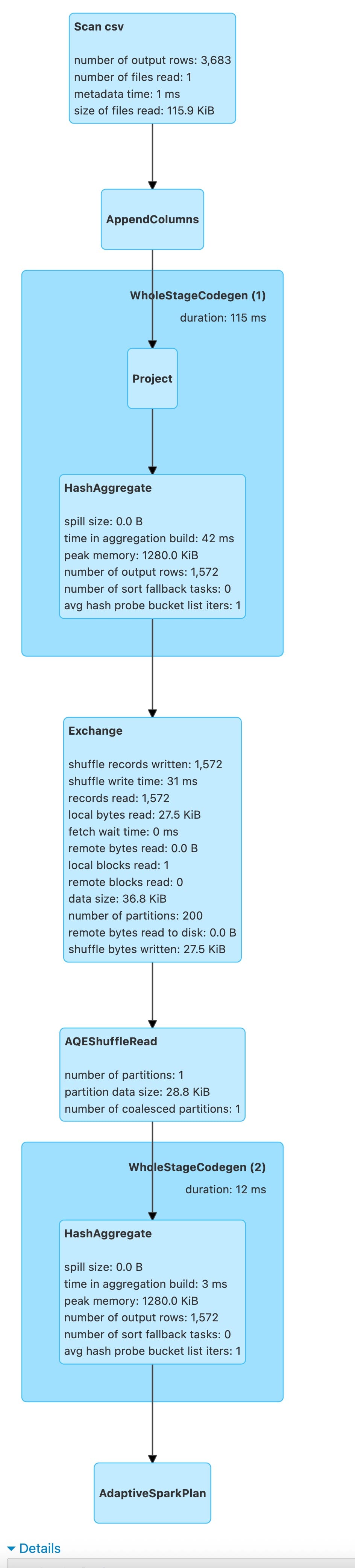
== Physical Plan ==
AdaptiveSparkPlan (13)
+- == Final Plan ==
   * HashAggregate (8)
   +- AQEShuffleRead (7)
      +- ShuffleQueryStage (6), Statistics(sizeInBytes=36.8 KiB, rowCount=1.57E+3)
         +- Exchange (5)
            +- * HashAggregate (4)
               +- * Project (3)
                  +- AppendColumns (2)
                     +- Scan csv  (1)
+- == Initial Plan ==
   HashAggregate (12)
   +- Exchange (11)
      +- HashAggregate (10)
         +- Project (9)
            +- AppendColumns (2)
               +- Scan csv  (1)
This physical plan demonstrates Adaptive Query Execution (AQE), a Spark optimisation feature that adjusts query execution plans dynamically at runtime based on actual data statistics collected during execution.
Structure Overview
The plan shows two versions:
- Initial Plan: The original execution plan created before query execution
- Final Plan: The optimized plan after runtime adaptations
Execution Flow (Bottom-Up)
Stage 1: Data Reading and Preparation
Scan csv (1)
- The query begins by reading data from a CSV file
- This is the data source for the entire query
- Spark reads the file in distributed fashion across executors
AppendColumns (2)
- This operation adds new columns to the DataFrame
- Typically results from Dataset API operations that involve lambda functions or user-defined transformations
- The columns being appended are computed based on existing data
Project (3)
- Performs column projection, selecting only the columns needed for downstream operations
- This is an optimization to reduce memory footprint and data transfer
- Unnecessary columns are dropped early in the pipeline
Stage 2: Partial Aggregation
HashAggregate (4) - Marked with asterisk (*)
- This is a partial (local) aggregation performed on each partition before shuffling
- The asterisk indicates WholeStageCodegen is enabled, meaning multiple operators are fused into a single optimized code block for better CPU efficiency
- Each executor computes partial aggregates for its local data partitions
- This significantly reduces the amount of data that needs to be shuffled across the network
- For example, if counting rows by key, each partition would produce local counts per key
Stage 3: Data Redistribution
Exchange (5)
- This is a shuffle operation that redistributes data across the cluster
- Data is repartitioned based on grouping keys so that all records with the same key end up on the same executor
- This is the most expensive operation in this plan due to network transfer and disk I/O
ShuffleQueryStage (6)
- This represents a query stage boundary in AQE
- Spark materializes the shuffle output and collects runtime statistics:
- sizeInBytes=36.8 KiB: The shuffle produced only 36.8 kilobytes of data
- rowCount=1.57E+3: Approximately 1,570 rows after partial aggregation
- These statistics are crucial for adaptive optimizations
- The stage completes before the next stage begins, allowing Spark to make informed decisions
Stage 4: Adaptive Optimization
AQEShuffleRead (7)
- This is an adaptive shuffle reader that adjusts how shuffle data is consumed
- Based on the statistics from ShuffleQueryStage, AQE can apply optimizations such as:
- Coalescing shuffle partitions: If shuffle output is small (as in this case with 36.8 KiB), Spark automatically reduces the number of partitions to avoid having many tiny tasks
- Partition skew handling: Redistributing work if some partitions are much larger than others
- Dynamic partition pruning: Eliminating unnecessary partitions based on runtime information
Stage 5: Final Aggregation
HashAggregate (8) - Marked with asterisk (*)
- This is the final (global) aggregation that combines the partial aggregates
- Each executor receives all data for specific keys and computes the final aggregate results
- WholeStageCodegen is applied for optimized execution
- This produces the final query results
Key Differences: Initial vs Final Plan
Initial Plan Characteristics
- No asterisks: WholeStageCodegen wasn’t shown in the initial plan
- Simple Exchange: Standard shuffle without adaptive features
- No query stages: No intermediate materialization points
- No statistics: Execution planned without runtime data knowledge
Final Plan Enhancements
- WholeStageCodegen enabled: HashAggregate operators marked with (*) indicate compiled code generation
- Query stage boundaries: Execution divided into stages with ShuffleQueryStage
- Runtime statistics collection: Actual data size and row counts captured
- Adaptive shuffle read: AQEShuffleRead replaces simple shuffle consumption
- Dynamic optimizations: Plan adjusted based on the discovered 36.8 KiB shuffle size
Runtime Optimizations Applied
Based on the statistics sizeInBytes=36.8 KiB, rowCount=1.57E+3, AQE likely applied:
-
Partition Coalescing: The default shuffle partition count (usually 200) was likely reduced because 36.8 KiB is very small. Instead of 200 tiny partitions, Spark may have coalesced them into just a few partitions, reducing task overhead.
-
WholeStageCodegen: Multiple physical operators are compiled into a single optimized Java bytecode function, eliminating virtual function calls and improving CPU cache utilization.
-
Reduced Task Overhead: Fewer partitions mean fewer tasks to schedule, reducing coordination overhead.
Why This Matters
Without AQE: Spark would use the default 200 shuffle partitions even for 36.8 KiB of data, creating 200 tiny tasks with overhead far exceeding actual work.
With AQE: Spark observes the small shuffle size at runtime and automatically coalesces partitions, potentially creating just 1-5 tasks instead of 200, dramatically improving performance.
Performance Implications
This query likely completes much faster with AQE because:
- Fewer tasks to schedule and coordinate
- Better resource utilization with appropriately sized tasks
- Reduced overhead from task serialization and deserialization
- More efficient final aggregation with optimal parallelism
The small shuffle size (36.8 KiB) suggests the partial aggregation was highly effective, reducing data from potentially much larger input to a very compact intermediate result.
Use of aggregates
aggapplies multiple aggregate functions to grouped data.as[Type]ensures type safety for aggregate results- Final
maptransforms tuple into case class
ratingsDS.printSchema()
root
 |-- userId: integer (nullable = true)
 |-- movieId: integer (nullable = true)
 |-- rating: double (nullable = true)
 |-- timestamp: integer (nullable = true)
import org.apache.spark.sql.functions._

ratingsDS.groupByKey(_.movieId).agg(
    count("*").as("Count").as[Long],
    max("rating").as("maximum rating").as[Long],
    min("rating").as("minimum rating").as[Long],
    avg("rating").as("avarage rating").as[Long]
).show(3)
+---+-----+--------------+--------------+------------------+
|key|Count|maximum rating|minimum rating|    avarage rating|
+---+-----+--------------+--------------+------------------+
| 70|   55|           5.0|           1.0|3.5090909090909093|
|157|   11|           5.0|           1.5|2.8636363636363638|
|362|   34|           5.0|           1.0|3.5294117647058822|
+---+-----+--------------+--------------+------------------+
only showing top 3 rows


import org.apache.spark.sql.functions._
The shuffle dependency is caused by groupByKey(_.movieId).
Why groupByKey causes a shuffle:
groupByKey is a wide transformation that requires shuffling because:
- Data Redistribution Required: Records with the same
movieIdneed to be co-located on the same partition for aggregation, but they’re initially scattered across multiple partitions - Network Transfer: - Before: Ratings for movieId=1 might exist on partitions 0, 2, 5, 7, etc. - After: All ratings for movieId=1 must be on a single partition - This requires moving data across the network between executors
- Stage Boundary: Spark creates a new stage to perform the aggregation after the shuffle completes
The Flow:
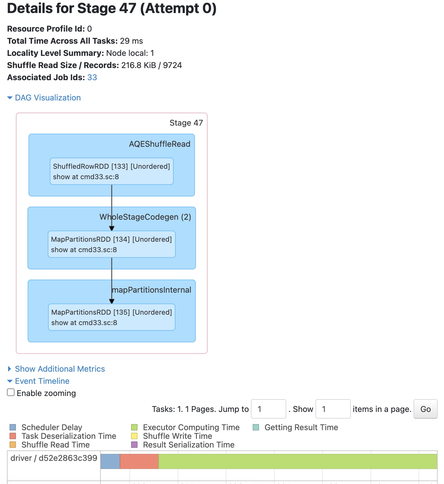
  Previous Stage → Shuffle Write (by movieId hash)
                        ↓
                    [Network shuffle]
                        ↓
  Stage 47 → Shuffle Read (216.8 KiB / 9,724 records) ← RED BOUNDARY
           → Group records by movieId
           → Compute aggregations (count, max, min, avg)
           → show(3)
Why the shuffle is necessary:
The aggregations (count, max, min, avg) need to process all ratings for each movie together. Without shuffling, each partition would only see a partial view of the ratings, giving incorrect results.
Alternative: If you used
groupBywith DataFrame APIs orreduceByKey, Spark could optimise with a map-side combine, butgroupByKeyon Datasets always performs a complete shuffle.
groupBy
Simply
// Show groups with count
ratingsDS
  .groupBy("movieId")
  .count()
  .show()
+-------+-----+
|movieId|count|
+-------+-----+
|     70|   55|
|    157|   11|
|    362|   34|
|    457|  190|
|    673|   53|
|   1029|   35|
|   1030|   15|
|   1032|   40|
|   1092|   47|
|   1256|   23|
|   1552|   59|
|   1580|  165|
|   1620|   13|
|   1732|  106|
|   2115|  108|
|   2116|   15|
|   2366|   25|
|   2414|   11|
|   2478|   26|
|   2716|  120|
+-------+-----+
only showing top 20 rows
aggapplies multiple aggregate functions to grouped data.as[Type]ensures type safety for aggregate results- Final
maptransforms tuple into case class
import org.apache.spark.sql.functions._

val ratingStats = ratingsDS
  .groupBy("movieId")
  .agg(
    count("*").as("Count"),
    max("rating").as("maximum rating"),
    min("rating").as("minimum rating"),
    avg("rating").as("average rating")
  )
import org.apache.spark.sql.functions._
ratingStats: DataFrame = [movieId: int, Count: bigint ... 3 more fields]
Benefits of groupBy Case
Without map-side combine:
- Would shuffle ALL rating records (potentially millions)
With map-side combine: Only shuffles aggregated stats per movieId (one row per movieId per partition)
The wide dependency still exists (shuffle is required), but map-side combine makes it much more efficient!
ratingStats.show(3)
+-------+-----+--------------+--------------+------------------+
|movieId|Count|maximum rating|minimum rating|    average rating|
+-------+-----+--------------+--------------+------------------+
|     70|   55|           5.0|           1.0|3.5090909090909093|
|    157|   11|           5.0|           1.5|2.8636363636363638|
|    362|   34|           5.0|           1.0|3.5294117647058822|
+-------+-----+--------------+--------------+------------------+
only showing top 3 rows
ratingStats.printSchema()
root
 |-- movieId: integer (nullable = true)
 |-- Count: long (nullable = false)
 |-- maximum rating: double (nullable = true)
 |-- minimum rating: double (nullable = true)
 |-- average rating: double (nullable = true)
flatMapGroups with Custom Logic
def flatMapGroups[U](f: (K, Iterator[V]) => TraversableOnce[U]): Dataset[U]
- Group-Wise Operations: Enables arbitrary operations on entire groups
- Stateful Processing: Can maintain state within group processing
- Flexible Output: Each group can produce 0, 1, or many output elements
For each group, applies filterFunny function
tagsDS
  .groupBy("movieId")
  .count()
  .show(3)
+-------+-----+
|movieId|count|
+-------+-----+
|  60756|    8|
|    431|    3|
|   1569|    3|
+-------+-----+
only showing top 3 rows
def filterFunny(label: Int, tags:Iterator[Tag]) = {
    tags.filter(_.tag.contains("funny"))
}

tagsDS.groupByKey(_.movieId).flatMapGroups(filterFunny).show()
+------+-------+----------------+----------+
|userId|movieId|             tag| timestamp|
+------+-------+----------------+----------+
|   357|     39|           funny|1348627869|
|   599|    296|           funny|1498456383|
|   599|    296|      very funny|1498456434|
|   599|   1732|           funny|1498456291|
|   477|   2706|       not funny|1244707227|
|    62|   2953|           funny|1525636885|
|    62|   3114|           funny|1525636913|
|     2|  60756|           funny|1445714994|
|    62|  60756|           funny|1528934381|
|   424|  60756|           funny|1457846127|
|    62|  68848|           funny|1527274322|
|   537|  69122|           funny|1424140317|
|    62|  71535|           funny|1529777194|
|    62|  88405|           funny|1525554868|
|    62|  99114|           funny|1526078778|
|   119| 101142|           funny|1436563067|
|   567| 106766|           funny|1525283917|
|    62| 107348|stupid but funny|1528935013|
|   567| 112852|           funny|1525285382|
|   177| 115617|      very funny|1435523876|
+------+-------+----------------+----------+
only showing top 20 rows


defined function filterFunny
mapGroups
The mapGroups transformation applies a user-defined function to each group produced by groupByKey. Unlike flatMapGroups, which can produce multiple results per group, mapGroups produces exactly one result per group.
def mapGroups[U](f: (K, Iterator[V]) => U)(implicit encoder: Encoder[U]): Dataset[U]
def countTags4Movie(m: Int, tags:Iterator[Tag]) = {
   (m, tags.size)
}
tagsDS.groupByKey(_.movieId).mapGroups(countTags4Movie).show(3)
+---+---+
| _1| _2|
+---+---+
|  1|  3|
|  2|  4|
|  3|  2|
+---+---+
only showing top 3 rows


defined function countTags4Movie
def findNoOfUserRatings(m:Int, users: Iterator[Rating]) = {
    val noOfUsersRatedTheMovie = users.size
    (m, noOfUsersRatedTheMovie)
}
ratingsDS.groupByKey(_.movieId).mapGroups(findNoOfUserRatings).show(2)
+---+---+
| _1| _2|
+---+---+
|  1|215|
|  2|110|
+---+---+
only showing top 2 rows


defined function findNoOfUserRatings
reduceGroups Operation
The reduceGroups operation applies a binary reduction function to all values within each group. This is similar to mapGroups but specifically for associative reduction operations where you combine values pairwise.
Signature:
def reduceGroups(f: (V, V) => V): Dataset[(K, V)]
Translation: Given a function that combines two values into one, apply it to all values in each group, returning one reduced value per group along with the key.
for example1:
case class Sale(product: String, amount: BigInt)
defined class Sale
val sales = Seq(
  Sale("Car", 10),
  Sale("Car", 20),
  Sale("Truck", 5),
  Sale("Bike", 15),
  Sale("Truck", 7)
).toDS()
sales: Dataset[Sale] = [product: string, amount: decimal(38,0)]
// reduceGroups: Sum amounts by product
def sumSales(s1: Sale, s2: Sale): Sale = {
  Sale(s1.product, s1.amount + s2.amount)
}

val totalsByProduct: Dataset[(String, Sale)] = sales
  .groupByKey(_.product)
  .reduceGroups(sumSales)
defined function sumSales
totalsByProduct: Dataset[(String, Sale)] = [key: string, ReduceAggregator(ammonite.$sess.cmd66$Helper$Sale): struct<product: string, amount: decimal(38,0)>]
for ((key, sale) <- totalsByProduct.collect()) {
  println(s"Key: $key, Product: ${sale.product}, Amount: ${sale.amount}")
}
Key: Car, Product: Car, Amount: 30
Key: Truck, Product: Truck, Amount: 12
Key: Bike, Product: Bike, Amount: 15
val totSales = totalsByProduct.first()._2
s"total sales of the ${totSales.product} is ${totSales.amount}"
totSales: Sale = Sale(product = "Car", amount = 30)
res70_1: String = "total sales of the Car is 30"
Summary:
In this notebook, used
- Scala
- Spark 3.3.1
scala.util.Properties.javaVersion
scala.util.Properties.versionMsg
res73_0: String = "17.0.17"
res73_1: String = "Scala library version 2.13.17 -- Copyright 2002-2025, LAMP/EPFL and Lightbend, Inc. dba Akka"
Stop the notebook
spark.stop()