Scala 2 Closures and Higher-Order Functions

Explore comprehensive Scala 2 functional programming fundamentals grounded in mathematical theory. This guide covers pure functions that ensure determinism and referential transparency, enabling equational reasoning and safe parallelization. Discover higher-order functions like map, filter, and fold that accept or return functions as first-class values. Master function composition techniques using compose and andThen operators to build complex pipelines. Learn currying—the mathematical transformation of multi-argument functions into sequences of single-argument functions. Understand immutability principles, side-effect elimination, and how these concepts form the backbone of scalable, testable Scala applications through category theory and lambda calculus foundations.

---

• Pure Functions
  • Mathematical Definition
  • Formal Definition
  • Mathematical Properties
  • Substitution Model
  • Pure Functions in Mathematics
  • Key Benefits of Pure Functions
• Higher-Order Functions
  • HOF Mathematical Definition
  • Type Theory Foundation of HOF
    • Example 1: Map - The Functor HOF
    • Example 2: Filter - Predicate-Based Selection
    • Example 3: Fold - Reduction Operations
      • foldr - right-associative fold
      • foldl - left-associative fold
      • Comparing foldr vs foldl
      • Insights:
    • Example 4: Custom HOFs
    • Composition in Scala
  • HOF Mathematical Properties
  • For-Comprehensions and HOFs
  • Type Signatures of Common HOFs
• Currying
  • Lambda Calculus Foundation
  • Uncurrying
  • Code Examples
    • Example 1: Manual Currying
    • Example 2: Scala’s Built-in Currying
    • Example 3: Converting Between Curried and Uncurried
• Scala Type Classes
  • Implicit Resolution
  • Example from the Cats book:
  • Implicit Scope
  • Key Benefits

---

Functional Programming (FP) is a programming paradigm based on mathematical functions where computation is treated as the evaluation of mathematical functions avoiding changing state and mutable data. This guide explores five fundamental FP concepts in Scala 2 with their mathematical foundations.

Core Principles of Functional Programming

1. Functions are first-class values: Functions can be passed as arguments, returned from other functions, and assigned to variables
2. Immutability: Data structures don’t change after creation
3. No side effects: Pure functions don’t modify external state
4. Referential Transparency: Expressions can be replaced by their values without changing program behavior

Pure Functions

Mathematical Definition

A pure function is a mathematical function where:

\[f: A \rightarrow B\]

Such that:

1. Determinism: $\forall x \in A, f(x)$ always produces the same output $y \in B$
2. No Side Effects: $f$ doesn’t modify any state outside its scope
3. Referential Transparency: For any program $p$, all occurrences of $f(x)$ can be replaced by its result without changing $p$’s meaning

Formal Definition

Referential Transparency (RT): An expression $e$ is referentially transparent if, for all programs $p$, all occurrences of $e$ in $p$ can be replaced by the result of evaluating $e$ without affecting the meaning of $p$.¹

Purity: A function $f$ is pure if the expression $f(x)$ is referentially transparent for all referentially transparent $x$.¹

Mathematical Properties

---
config:
  look: neo
  theme: default
---
graph TB
    A[Pure Function Properties] --> B[Determinism]
    A --> C[No Side Effects]
    A --> D[Referential Transparency]
    B --> E["∀x: f(x) = constant"]
    C --> F["No I/O, mutations, or exceptions"]
    D --> G["Can substitute f(x) with its result"]
    style A fill:#e1f5ff
    style B fill:#fff4e1
    style C fill:#fff4e1
    style D fill:#fff4e1

Substitution Model

Pure functions enable equational reasoning through the substitution model:

\[\begin{align} \text{Given: } & f(x) = x^2 \\ \text{Then: } & f(3) + f(3) \\ & = 9 + f(3) \quad \text{(substitute first)} \\ & = 9 + 9 \quad \text{(substitute second)} \\ & = 18 \end{align}\]

for example,

// Pure Function - Always returns the same output for the same input
def square(x: Int): Int = x * x

// Test purity
val result1 = square(5)  // 25
val result2 = square(5)  // 25
// result1 == result2 always true

defined function square
result1: Int = 25
result2: Int = 25

Mathematical proof:

square(5) = 5 * 5 = 25

NOTE: Can always replace square(5) with 25

Pure function using internal mutable state (hidden from outside).

Pure Functions in Mathematics

Mathematical Concept	Scala Example	Property
$f(x) = x + 1$	def inc(x: Int) = x + 1	Successor function
$f(x, y) = x + y$	def add(x: Int, y: Int) = x + y	Addition
$f(x) = x^2$	def square(x: Int) = x * x	Quadratic
$f(s) = |s|$	def length(s: String) = s.length	String length
$f(x) = e^x$	def exp(x: Double) = math.exp(x)	Exponential

Key Benefits of Pure Functions

1. Testability: Easy to test - same input always produces the same output
2. Parallelisation: Can safely run in parallel (no shared mutable state)
3. Memoization: Results can be cached
4. Reasoning: Enable algebraic reasoning and equational substitution
5. Composition: Can combine pure functions to create complex behaviour

---
config:
  look: neo
  theme: default
---
mindmap
  root((Pure Functions))
    Benefits
      Easy Testing
        Predictable
        No Mocks Needed
      Parallelization
        Thread Safe
        No Race Conditions
      Caching
        Memoization
        Performance
    Properties
      Deterministic
      No Side Effects
      Referential Transparency
    Applications
      Mathematical Computations
      Data Transformations
      Functional Pipelines

---

Higher-Order Functions

Morphisms are simply arrows or mappings between objects in a category. Think of them as generalized functions. When we say “objects are types and morphisms are functions”:

• Objects = Types (Int, String, List[A], etc.)
• Morphisms = Functions between those types

def length: String => Int

This is a morphism from the object String to the object Int.

String —-length—-> Int (object) (morphism) (object)

A higher-order function like map is a morphism in a “higher” category:

def map[A, B](f: A => B): List[A] => List[B]
// or curried version
def map[A, B](f: A => B)(xs: List[A]): List[B]

Here:

• Objects are themselves function types: (A => B), (List[A] => List[B])
• Morphism is map, which maps between these function objects

(A => B) ----map----> (List[A] => List[B])

HOF Mathematical Definition

A higher-order function (HOF) is a function that:

1. Takes one or more functions as arguments, or
2. Returns a function as its result

\[\text{HOF}: (A \rightarrow B) \rightarrow C \text{ or } A \rightarrow (B \rightarrow C)\]

In category theory, HOFs are morphisms in the category of functions where objects are types and morphisms are functions.²

Type Theory Foundation of HOF

In the simply typed lambda calculus, if $\tau_1, \tau_2, \tau_3$ are types:

\[f: (\tau_1 \rightarrow \tau_2) \rightarrow \tau_3 \text{ is a HOF}\]

This means $f$ accepts a function of type $\tau_1 \rightarrow \tau_2$ and produces a value of type $\tau_3$.

Examples

1. Map operation (Functor)
2. Filter operation
3. Fold operation:

Example 1: Map - The Functor HOF³

Map operation (Functor):

\[\text{map}: (A \rightarrow B) \rightarrow [A] \rightarrow [B]\]

This reads as: “map takes a function from A to B, then takes a list of A’s, and returns a list of B’s”.

The arrows represent currying - map doesn’t take all arguments at once, but returns functions:

• Takes (A → B) - a function from type A to type B
• Returns a function that takes [A] - a list of A’s
• Which returns [B] - a list of B’s

Behaviour:

\[\text{map}\ f\ [x_1, x_2, ..., x_n] = [f(x_1), f(x_2), ..., f(x_n)]\]

Apply function f to each element in the list.

The map applies a function to each element

def map[A, B](f: A => B)(xs: List[A]): List[B] = xs match {
  case Nil => Nil
  case head :: tail => f(head) :: map(f)(tail)
}

Type Parameters: [A, B] - generic types matching the math notation

Curried Syntax: Two parameter lists (f: A => B)(xs: List[A]) implements the curried arrows:

• First takes function f: A => B (matching A → B)
• Then takes list xs: List[A] (matching [A])
• Returns List[B] (matching [B])

The recursive case implements the mathematical definition:

• f(head) - apply f to first element (like f(x₁))
• map(f)(tail) - recursively map over remaining elements (like [f(x₂), ..., f(xₙ)])
• :: - cons operator joins them together

Example execution is

map(x => x * 2)(List(1, 2, 3))

Traces to:

f(1) :: map(f)(List(2, 3))
2 :: f(2) :: map(f)(List(3))
2 :: 4 :: f(3) :: map(f)(Nil)
2 :: 4 :: 6 :: Nil
List(2, 4, 6)

This matches the math: map (*2) [1,2,3] = [2, 4, 6] ✓

// Using map
val numbers = List(1, 2, 3)
val squared = map((x: Int) => x * 2)(numbers)
// Result: List(1, 4, 9, 16, 25)

// Mathematical property (Functor law):
// map(id) == id
// map(f ∘ g) == map(f) ∘ map(g)

numbers: List[Int] = List(1, 2, 3)
squared: List[Int] = List(2, 4, 6)

Scala standard library usage

val nums = List(1, 2, 3)

// map with named function
def double(x: Int): Int = x * 2
nums.map(double)  // List(2, 4, 6, 8, 10)

nums: List[Int] = List(1, 2, 3)
defined function double
res14_2: List[Int] = List(2, 4, 6)

Example 2: Filter - Predicate-Based Selection³

filter keeps elements satisfying a predicate

\[\text{filter}: (A \rightarrow \text{Bool}) \rightarrow [A] \rightarrow [A]\]

This reads as: “filter takes a predicate function from A to Boolean, then takes a list of A’s, and returns a list of A’s”

Key difference from map: the input and output list types are the same ([A] → [A]) because we’re selecting elements, not transforming them.

The currying structure:

• Takes (A → Bool) - a predicate function that tests elements
• Returns a function that takes [A] - a list of A’s
• Which returns [A] - a filtered list of A’s

Behaviour (List Comprehension):

This is list comprehension notation meaning: “build a list containing all elements x drawn from xs where the predicate p(x) is true”

\[\text{filter}\ p\ xs = [x\ |\ x \leftarrow xs, p(x)]\]

def filter[A](p: A => Boolean)(xs: List[A]): List[A] = xs match {
  case Nil => Nil
  case head :: tail => 
    if (p(head)) head :: filter(p)(tail)
    else filter(p)(tail)
}

defined function filter

Type Parameter: [A] - single generic type (input and output are same type)

Curried Syntax: (p: A => Boolean)(xs: List[A]) implements:

• First takes predicate p: A => Boolean (matching A → Bool)
• Then takes list xs: List[A] (matching [A])
• Returns List[A] (matching [A])

Pattern Matching Implementation:

The recursive logic implements the list comprehension:

• Test: if (p(head)) - checks if predicate holds for current element
• Include: head :: filter(p)(tail) - keep element and continue
• Exclude: filter(p)(tail) - skip element and continue
• Eventually builds a list of only elements where p(x) was true

// Using filter
val numbers = List(1, 2, 3, 4, 5, 6, 7, 8, 9, 10)

// Keep even numbers
val evens = filter((x: Int) => x % 2 == 0)(numbers)
// Result: List(2, 4, 6, 8, 10)

// Mathematical definition as list comprehension:
// filter p xs = [x | x ← xs, p x]

numbers: List[Int] = List(1, 2, 3, 4, 5, 6, 7, 8, 9, 10)
evens: List[Int] = List(2, 4, 6, 8, 10)

Example Execution

filter(x => x > 2)(List(1, 2, 3, 4))

Traces to:

p(1) = false → filter(p)(List(2, 3, 4))
p(2) = false → filter(p)(List(3, 4))
p(3) = true  → 3 :: filter(p)(List(4))
p(4) = true  → 3 :: 4 :: filter(p)(Nil)
3 :: 4 :: Nil
List(3, 4)

Scala Standard library usage:

// Practical examples
val numbers = List(-3, -2, -1, 0, 1, 2, 3, 4, 5)

// Filter positive numbers
numbers.filter(_ > 0)  // List(1, 2, 3)

// Filter even numbers
numbers.filter(x => x % 2 == 0)  // List(-2, 0, 2, 4)

// Chain filter operations
numbers
  .filter(_ > 0)        // List(1, 2, 3, 4, 5)
  .filter(_ % 2 == 0)   // List(2, 4)

numbers: List[Int] = List(-3, -2, -1, 0, 1, 2, 3, 4, 5)
res18_1: List[Int] = List(1, 2, 3, 4, 5)
res18_2: List[Int] = List(-2, 0, 2, 4)
res18_3: List[Int] = List(2, 4)

This matches the math: \(\text{filter}\ (>2)\ [1,2,3,4] = [x\ |\ x \leftarrow [1,2,3,4], x > 2] = [3, 4]\)

Example 3: Fold - Reduction Operations³

foldr - right-associative fold

\[\text{foldr}: (A \rightarrow B \rightarrow B) \rightarrow B \rightarrow [A] \rightarrow B\]

This reads as: “foldr takes a combining function, then an initial value, then a list, and returns a single accumulated value”

The currying structure (three levels):

• Takes (A → B → B) - a combining function that takes an element of type A and an accumulator of type B, returning a new B
• Then takes B - an initial/accumulator value
• Then takes [A] - a list of A’s
• Returns B - a single folded result

Behaviour (Right-Associative):

\[\text{foldr}\ (\oplus)\ a\ [x_1, x_2, ..., x_n] = x_1 \oplus (x_2 \oplus ... (x_n \oplus a))\]

Works right-to-left, with parentheses showing association from the right. The rightmost element xₙ is combined with the initial value first, then that result is combined with xₙ₋₁, and so on.

def foldr[A, B](f: (A, B) => B)(z: B)(xs: List[A]): B = xs match {
  case Nil => z
  case head :: tail => f(head, foldr(f)(z)(tail))
}

// Mathematical notation:
// foldr (⊕) a [x₁, x₂, ..., xₙ] = x₁ ⊕ (x₂ ⊕ ... (xₙ ⊕ a))

defined function foldr

Type Parameters: [A, B] - two types (list elements and accumulator can differ)

Three Parameter Lists (Curried):

• (f: (A, B) => B) - combining function (matching A → B → B)
• (z: B) - initial/”zero” value (matching the B)
• (xs: List[A]) - input list (matching [A])
• Returns B - folded result

The recursive case implements right-associativity:

• foldr(f)(z)(tail) - first recursively fold the tail (processes right side)
• f(head, ...) - then combine head with that result (processes left side)
• This creates the structure: head ⊕ (recursive_result)

Example Execution

// Practical fold examples
val numbers = List(1, 2, 3, 4, 5)
// Product using foldRight
val product = numbers.foldRight(1)(_ * _)  // 120
// Evaluation: 1 * (2 * (3 * (4 * (5 * 1))))

numbers: List[Int] = List(1, 2, 3, 4, 5)
product: Int = 120

see the trace below for the following

foldr((x: Int, acc: Int) => x + acc)(0)(List(1, 2, 3))

res34: Int = 6

Traces to:

f(1, foldr(f)(0)(List(2, 3)))
f(1, f(2, foldr(f)(0)(List(3))))
f(1, f(2, f(3, foldr(f)(0)(Nil))))
f(1, f(2, f(3, 0)))
f(1, f(2, 3))
f(1, 5)
6

This matches the math: \(\text{foldr}\ (+)\ 0\ [1,2,3] = 1 + (2 + (3 + 0)) = 1 + (2 + 3) = 1 + 5 = 6\) ✓

Visualising Right Association

For foldr (⊕) a [x₁, x₂, x₃]:

    x₁ ⊕ (x₂ ⊕ (x₃ ⊕ a))
    │      │      │
    │      │      └─ combines first
    │      └──────── combines second  
    └─────────────── combines last

foldl - left-associative fold

\[\text{foldl}: (B \rightarrow A \rightarrow B) \rightarrow B \rightarrow [A] \rightarrow B\]

This reads as: “foldl takes a combining function, then an initial value, then a list, and returns a single accumulated value”

The currying structure (three levels):

• Takes (B → A → B) - a combining function that takes an accumulator of type B and an element of type A, returning a new B
  • Note: Arguments are reversed compared to foldr!
• Then takes B - an initial/accumulator value
• Then takes [A] - a list of A’s
• Returns B - a single folded result

Behaviour (Left-Associative):

\[\text{foldl}\ (\oplus)\ a\ [x_1, x_2, ..., x_n] = ((...((a \oplus x_1) \oplus x_2) ...) \oplus x_n)\]

Works left-to-right, with parentheses showing association from the left. The leftmost element x₁ is combined with the initial value a first, then that result is combined with x₂, and so on.

// foldl - left-associative fold
def foldl[A, B](f: (B, A) => B)(z: B)(xs: List[A]): B = xs match {
  case Nil => z
  case head :: tail => foldl(f)(f(z, head))(tail)
}

// Mathematical notation:
// foldl (⊕) a [x₁, x₂, ..., xₙ] = (((a ⊕ x₁) ⊕ x₂) ... ⊕ xₙ)

defined function foldl

Type Parameters: [A, B] - two types (list elements and accumulator can differ)

Three Parameter Lists (Curried):

• (f: (B, A) => B) - combining function with accumulator first (matching B → A → B)
• (z: B) - initial/”zero” value (matching the B)
• (xs: List[A]) - input list (matching [A])
• Returns B - folded result

Example Execution

The recursive case implements left-associativity:

• f(z, head) - first combine accumulator with head (processes left side)
• foldl(f)(...)(tail) - then recursively fold tail with new accumulator
• This creates the structure: (previous_result) ⊕ head

foldl((acc: Int, x: Int) => acc + x)(0)(List(1, 2, 3)) // traced

res36: Int = 6

Traces to:

foldl(f)(f(0, 1))(List(2, 3))
foldl(f)(1)(List(2, 3))
foldl(f)(f(1, 2))(List(3))
foldl(f)(3)(List(3))
foldl(f)(f(3, 3))(Nil)
foldl(f)(6)(Nil)
6

This matches the math: \(\text{foldl}\ (+)\ 0\ [1,2,3] = ((0 + 1) + 2) + 3 = (1 + 2) + 3 = 3 + 3 = 6\) ✓

Visualising Left Association

For foldl (⊕) a [x₁, x₂, x₃]:

    ((a ⊕ x₁) ⊕ x₂) ⊕ x₃
     │         │       │
     │         │       └─ combines last
     │         └──────── combines second  
     └─────────────────── combines first

For example, Building a reversed list with foldLeft

val reversed = numbers.foldLeft(List.empty[Int])((acc, x) => x :: acc)
// Result: List(5, 4, 3, 2, 1)

reversed: List[Int] = List(5, 4, 3, 2, 1)

Scala Standard library usage:

// Practical fold examples
val numbers = List(1, 2, 3, 4, 5)

// Sum using foldLeft
val sum = numbers.foldLeft(0)(_ + _)  // 15
// Evaluation: ((((0 + 1) + 2) + 3) + 4) + 5

// Product using foldRight
val product = numbers.foldRight(1)(_ * _)  // 120
// Evaluation: 1 * (2 * (3 * (4 * (5 * 1))))

// Building a reversed list with foldLeft
val reversed = numbers.foldLeft(List.empty[Int])((acc, x) => x :: acc)
// Result: List(5, 4, 3, 2, 1)

numbers: List[Int] = List(1, 2, 3, 4, 5)
sum: Int = 15
product: Int = 120
reversed: List[Int] = List(5, 4, 3, 2, 1)

Defining common operations with fold

def sum(xs: List[Int]): Int = xs.foldRight(0)(_ + _)

def product(xs: List[Int]): Int = xs.foldRight(1)(_ * _)

def length[A](xs: List[A]): Int = xs.foldRight(0)((_, acc) => acc + 1)

def concatenate[A](xss: List[List[A]]): List[A] = xss.foldRight(List.empty[A])(_ ++ _)

// Example usage
sum(List(1, 2, 3, 4, 5))           // 15
product(List(1, 2, 3, 4, 5))       // 120
length(List('a', 'b', 'c'))        // 3
concatenate(List(List(1,2), List(3,4)))  // List(1, 2, 3, 4)

defined function sum
defined function product
defined function length
defined function concatenate
res37_4: Int = 15
res37_5: Int = 120
res37_6: Int = 3
res37_7: List[Int] = List(1, 2, 3, 4)

Comparing foldr vs foldl

foldr: x₁ ⊕ (x₂ ⊕ (x₃ ⊕ a))

• Right-associative
• Processes right side first (via recursion)
• Function signature: (A, B) => B

foldl: ((a ⊕ x₁) ⊕ x₂) ⊕ x₃

• Left-associative
• Processes left side first (via accumulator)
• Function signature: (B, A) => B

Example Where Order Matters

// Division is NOT associative
foldr((x: Int, acc: Int) => x / acc)(1)(List(8, 4, 2))
// 8 / (4 / (2 / 1)) = 8 / (4 / 2) = 8 / 2 = 4

foldl((acc: Int, x: Int) => acc / x)(64)(List(4, 2, 2))
// ((64 / 4) / 2) / 2 = (16 / 2) / 2 = 8 / 2 = 4

res28_0: Int = 4
res28_1: Int = 4

Different structure, potentially different results!

Example: Building a Reversed List

foldl((acc: List[Int], x: Int) => x :: acc)(Nil)(List(1, 2, 3))

res29: List[Int] = List(3, 2, 1)

((Nil :: 1) :: 2) :: 3
(List(1) :: 2) :: 3
List(2, 1) :: 3
List(3, 2, 1)

This reverses the list! In fact, foldl (flip (::)) Nil xs = reverse xs

Insights:

• foldl is tail-recursive in this implementation - the recursive call is the last operation, making it more memory efficient
• Left-associative: processes list from left to right via accumulator
• Accumulator-first: the function takes (B, A) not (A, B) - accumulator is first argument
• For associative operations (like +, *), foldr and foldl produce the same result
• For non-associative operations (like -, /, ::) they produce different results
• In practice: foldl is often preferred for efficiency (tail-recursive), but foldr works on infinite lists

Example 4: Custom HOFs

A HOF that applies a function n times.

The applyNTimes function implements repeated function composition or function exponentiation:

\[f^n(x) = \underbrace{f \circ f \circ \cdots \circ f}_{n \text{ times}}(x)\]

More explicitly:

• $f^0(x) = x$ (identity - apply 0 times)
• $f^1(x) = f(x)$ (apply once)
• $f^2(x) = f(f(x))$ (apply twice)
• $f^3(x) = f(f(f(x)))$ (apply three times)
• $f^n(x) = f(f^{n-1}(x))$ (recursive definition)

in Mathematics

\[\text{applyNTimes}: (A \rightarrow A) \rightarrow \mathbb{N} \rightarrow (A \rightarrow A)\]

Reads as: “Takes an endomorphism (function from A to itself) and a natural number, returns another endomorphism”

Type Analysis

• Input 1: f: A => A - an endomorphism (function that maps type A to itself)
• Input 2: n: Int - number of times to compose f
• Output: A => A - a new function that applies f exactly n times

The loop helper function:

\[\text{loop}(x, k) = \begin{cases} x & \text{if } k \leq 0 \\ \text{loop}(f(x), k-1) & \text{if } k > 0 \end{cases}\]

This implements: $\text{loop}(x, n) = f^n(x)$

def applyNTimes[A](f: A => A, n: Int): A => A = {
  def loop(x: A, remaining: Int): A = {
    if (remaining <= 0) x
    else loop(f(x), remaining - 1)
  }
  (x: A) => loop(x, n)
}

defined function applyNTimes

Execution trace for loop(x, 3):

loop(x, 3)
→ loop(f(x), 2)
→ loop(f(f(x)), 1)
→ loop(f(f(f(x))), 0)
→ f(f(f(x)))

val increment: Int => Int = x => x + 1

val addFive = applyNTimes(increment, 5)
// addFive is equivalent to: x => x + 1 + 1 + 1 + 1 + 1

addFive(10)  // Output: 15

increment: Int => Int = ammonite.$sess.cmd40$Helper$$Lambda$2754/0x000000012c898bc8@7d57e5ae
addFive: Int => Int = ammonite.$sess.cmd38$Helper$$Lambda$2750/0x000000012c897908@612c3a59
res40_2: Int = 15

\[\begin{aligned} \text{addFive}(10) &= \text{increment}^5(10) \\ &=\text{increment}(\text{increment}(\text{increment}(\text{increment}(\text{increment}(10))))) \\ &=\text{increment}(\text{increment}(\text{increment}(\text{increment}(11)))) \\ &=\text{increment}(\text{increment}(\text{increment}(12))) \\ &=\text{increment}(\text{increment}(13)) \\ &=\text{increment}(14) \\ &= 15 \end{aligned}\]

Function design properties:

1: Identity Law

\(\text{applyNTimes}(f, 0) = \text{id}\) Where $\text{id}(x) = x$ for all $x$

val identityFunc = applyNTimes(increment, 0)
identityFunc(10)

identityFunc: Int => Int = ammonite.$sess.cmd38$Helper$$Lambda$2750/0x000000012c897908@6a7a462
res43_1: Int = 10

2: Composition Law

\[\text{applyNTimes}(f, m + n) = \text{applyNTimes}(f, m) \circ \text{applyNTimes}(f, n)\]

val add3 = applyNTimes(increment, 3)
val add5 = applyNTimes(increment, 5)
val add8 = applyNTimes(increment, 8)

// These are equivalent:
add8(10)           // 18
add5(add3(10))     // 18

add3: Int => Int = ammonite.$sess.cmd38$Helper$$Lambda$2750/0x000000012c897908@447f7c8f
add5: Int => Int = ammonite.$sess.cmd38$Helper$$Lambda$2750/0x000000012c897908@150f8d6c
add8: Int => Int = ammonite.$sess.cmd38$Helper$$Lambda$2750/0x000000012c897908@7ddc39a
res44_3: Int = 18
res44_4: Int = 18

3: Recursive Structure \(f^n = f \circ f^{n-1}\)

This is exactly what the loop function implements through tail recursion.

In category theory, applyNTimes works with endomorphisms in a category:

• Objects: Types (like Int, String, etc.)
• Morphisms: Functions between types
• Endomorphism: A morphism from an object to itself (A => A)

The function creates a monoid structure:

• Binary operation: Function composition $\circ$
• Identity element: $f^0 = \text{id}$
• Closure: $f^m \circ f^n = f^{m+n}$

Tail Recursion Optimisation

The loop function is tail-recursive because:

• The recursive call is the last operation
• No additional computation after the recursive call returns
• Scala compiler can optimise it to a loop (with @tailrec annotation)

import scala.annotation.tailrec

def applyNTimes[A](f: A => A, n: Int): A => A = {
  @tailrec
  def loop(x: A, remaining: Int): A = {
    if (remaining <= 0) x
    else loop(f(x), remaining - 1)
  }
  (x: A) => loop(x, n)
}

import scala.annotation.tailrec


defined function applyNTimes

Composition in Scala

Understanding Function Composition in Scala

Function composition forms a category:

Category of Types and Functions:

• Objects: Types (Int, String, Boolean, etc.)
• Morphisms: Functions between types
• Composition: Function composition operator
• Identity: Identity function for each type

Category Laws:

1. Associativity: $(f \circ g) \circ h = f \circ (g \circ h)$
2. Identity: $f \circ \text{id}_A = f = \text{id}_B \circ f$ for $f: A \to B$

This makes function composition a fundamental operation in functional programming.

In mathematics, function composition is denoted by the symbol $\circ$ (circle):

\[(f \circ g)(x) = f(g(x))\]

Read as: “f composed with g, applied to x, equals f of g of x”

Key points:

• Apply $g$ first to $x$
• Then apply $f$ to the result
• The right function ($g$) is applied first
• Composition flows right-to-left

x  →  [g]  →  g(x)  →  [f]  →  f(g(x))
      apply g first    then apply f

For composition $f \circ g$ to be valid: \(f: B \rightarrow C\) \(g: A \rightarrow B\) \(f \circ g: A \rightarrow C\)

The output type of $g$ must match the input type of $f$.

def compose[A, B, C](f: B => C, g: A => B): A => C = {
  (x: A) => f(g(x))
}

defined function compose

Type Analysis

Type signature: \(\text{compose}: (B \rightarrow C) \rightarrow (A \rightarrow B) \rightarrow (A \rightarrow C)\)

• Parameter 1: f: B => C - function that transforms B to C
• Parameter 2: g: A => B - function that transforms A to B
• Returns: A => C - a new function that transforms A to C

How It Works

The function returns a closure (lambda):

(x: A) => f(g(x))

This lambda:

1. Takes an argument x of type A
2. Applies g to get a value of type B
3. Applies f to get a final value of type C

Examples:

val addOne = (x: Int) => x + 1
val double = (x: Int) => x * 2
val addOneThenDouble = compose(double, addOne)
addOneThenDouble(5)

addOne: Int => Int = ammonite.$sess.cmd49$Helper$$Lambda$2790/0x000000012c8a4000@54d5fa77
double: Int => Int = ammonite.$sess.cmd49$Helper$$Lambda$2791/0x000000012c8a43e8@27a2a472
addOneThenDouble: Int => Int = ammonite.$sess.cmd47$Helper$$Lambda$2786/0x000000012c89ed08@7da32905
res49_3: Int = 12

Type flow:

• addOne: Int => Int (matches A => B where A=Int, B=Int)
• double: Int => Int (matches B => C where B=Int, C=Int)
• addOneThenDouble: Int => Int (resulting A => C)

Execution trace:

\[\begin{flalign*} \text{addOneThenDouble}(5) &= \text{double}(\text{addOne}(5)) \\ &= \text{double}(5 + 1) \\ &= \text{double}(6) \\ &= 6 \times 2 \\ &= 12 \end{flalign*}\]

Scala provides two composition methods in the standard library:

Concept	Mathematical	Scala compose	Scala andThen
Notation	$f \circ g$	f compose g	g andThen f
Meaning	$f(g(x))$	f(g(x))	f(x) then g
Flow	Right-to-left	Right-to-left	Left-to-right
Natural?	Math traditional	Math traditional	More intuitive

1: compose - Right-to-Left (Mathematical Order)

val f = addOne compose double
// Equivalent to: (x: Int) => addOne(double(x))

f: Int => Int = scala.Function1$$Lambda$2796/0x000000012c8a1118@28b3e02d

mathamatically

\(f = \text{addOne} \circ \text{double}\) \(f(x) = \text{addOne}(\text{double}(x))\)

Execution:

f(5)  // addOne(double(5))
      // = addOne(5 * 2)
      // = addOne(10)
      // = 10 + 1
      // = 11

Flow diagram:

5  →  [double]  →  10  →  [addOne]  →  11
      apply first       apply second

2: andThen - Left-to-Right (Pipeline Order)

val g = addOne andThen double
// Equivalent to: (x: Int) => double(addOne(x))

g: Int => Int = scala.Function1$$Lambda$766/0x000000012c5360b0@7d14a8aa

mathamatically

\(g = \text{double} \circ \text{addOne}\) \(g(x) = \text{double}(\text{addOne}(x))\)

Execution:

g(5)  // double(addOne(5))
      // = double(5 + 1)
      // = double(6)
      // = 6 * 2
      // = 12

Flow diagram:

5  →  [addOne]  →  6  →  [double]  →  12
      apply first      apply second

HOF Mathematical Properties

Property	Mathematical Form	Code Example
Map Composition	$\text{map}(f \circ g) = \text{map}(f) \circ \text{map}(g)$	xs.map(g).map(f) == xs.map(f compose g)
Map Identity	$\text{map}(\text{id}) = \text{id}$	xs.map(x => x) == xs
Filter Composition	$\text{filter}(p) \circ \text{filter}(q) = \text{filter}(q) \circ \text{filter}(p)$	xs.filter(p).filter(q) == xs.filter(q).filter(p)
Fold Fusion	$\text{map}(f) \circ \text{fold}(g)(z) = \text{fold}(g \circ f)(z)$	Optimization technique

For-Comprehensions and HOFs⁴

The for comprehension is syntactic sugar for HOF chains

for {
    x <- List(1,2,3)
    y <- List(10, 20)
    if x * y > 10 // Guard
} yield x * y

res53: List[Int] = List(20, 20, 40, 30, 60)

Desugars to:

List(1,2,3).flatMap(x => List(10,20).filter( y => x * y > 10).map( y => x * y))

res60: List[Int] = List(20, 20, 40, 30, 60)

Type Signatures of Common HOFs

Function	Type Signature	Description
map	[A, B](f: A => B): List[A] => List[B]	Apply function to each element
filter	[A](p: A => Boolean): List[A] => List[A]	Keep elements satisfying predicate
foldLeft	[A, B](z: B)(f: (B, A) => B): List[A] => B	Left-associative reduction
foldRight	[A, B](z: B)(f: (A, B) => B): List[A] => B	Right-associative reduction
flatMap	[A, B](f: A => List[B]): List[A] => List[B]	Map then flatten
find	[A](p: A => Boolean): List[A] => Option[A]	Find first matching element
exists	[A](p: A => Boolean): List[A] => Boolean	Check if any element matches
forall	[A](p: A => Boolean): List[A] => Boolean	Check if all elements match

Currying

Mathematically:

Currying is the transformation of a function with multiple arguments into a sequence of functions, each taking a single argument.⁵

Named after mathematician Haskell Curry, currying transforms:

\[f: A \times B \times C \rightarrow D\]

Into:

\[\text{curry}(f): A \rightarrow (B \rightarrow (C \rightarrow D))\]

This isomorphism is expressed as:

\[\text{Hom}(A \times B, C) \cong \text{Hom}(A, C^B)\]

Where $C^B$ denotes the exponential object (function type $B \rightarrow C$).

Lambda Calculus Foundation

In lambda calculus, currying is a natural consequence of functions only taking one argument:

\[\begin{align} \lambda xy.\ x + y &\equiv \lambda x.(\lambda y.\ x + y) \\ \text{apply to 3: } &(\lambda x.(\lambda y.\ x + y))\ 3 \\ &= \lambda y.\ 3 + y \end{align}\]

Uncurrying

The inverse transformation:

\[\text{uncurry}: (A \rightarrow (B \rightarrow C)) \rightarrow ((A \times B) \rightarrow C)\]

Code Examples

Example 1: Manual Currying⁵

// Regular multi-parameter function
def add(x: Int, y: Int, z: Int): Int = x + y + z

// Manually curried version
def addCurried(x: Int): Int => Int => Int = {
  (y: Int) => {
    (z: Int) => {
      x + y + z
    }
  }
}

// Using the curried version
val addFive = addCurried(5)        // Returns function: Int => Int => Int
val addFiveSeven = addFive(7)      // Returns function: Int => Int
val result = addFiveSeven(3)       // Returns: 15

// Or in one line:
addCurried(5)(7)(3)  // 15

// Mathematical evaluation:
// addCurried(5)(7)(3)
// = ((x => y => z => x+y+z)(5))(7)(3)
// = (y => z => 5+y+z)(7)(3)
// = (z => 5+7+z)(3)
// = 5+7+3 = 15

defined function add
defined function addCurried
addFive: Int => Int => Int = ammonite.$sess.cmd62$Helper$$Lambda$3713/0x000000012cb02650@6f83cc5f
addFiveSeven: Int => Int = ammonite.$sess.cmd62$Helper$$Lambda$3714/0x000000012cb02a18@21cb32c7
result: Int = 15
res62_5: Int = 15

Example 2: Scala’s Built-in Currying⁵

// Scala syntax for curried functions (multiple parameter lists)
def multiply(x: Int)(y: Int)(z: Int): Int = x * y * z

// Partial application at each level
val timesTen = multiply(10) _      // Int => Int => Int
val timesTenFive = timesTen(5)     // Int => Int
val result = timesTenFive(2)       // 100

// Can also apply all at once
multiply(10)(5)(2)  // 100

// Type signatures:
// multiply: (x: Int)(y: Int)(z: Int): Int
// multiply(10): Int => Int => Int
// multiply(10)(5): Int => Int
// multiply(10)(5)(2): Int

defined function multiply
timesTen: Int => Int => Int = ammonite.$sess.cmd63$Helper$$Lambda$3719/0x000000012cb03f68@48891e11
timesTenFive: Int => Int = ammonite.$sess.cmd63$Helper$$Lambda$3720/0x000000012cb04338@23033b53
result: Int = 100
res63_4: Int = 100

Example 3: Converting Between Curried and Uncurried¹

// Generic curry and uncurry functions

// Curry: Convert (A, B) => C to A => B => C
def curry[A, B, C](f: (A, B) => C): A => B => C = {
  (a: A) => (b: B) => f(a, b)
}

// Uncurry: Convert A => B => C to (A, B) => C
def uncurry[A, B, C](f: A => B => C): (A, B) => C = {
  (a: A, b: B) => f(a)(b)
}

// Example usage
val add: (Int, Int) => Int = (x, y) => x + y
val addCurried: Int => Int => Int = curry(add)
val addUncurried: (Int, Int) => Int = uncurry(addCurried)

// Test
add(3, 4)              // 7
addCurried(3)(4)       // 7
addUncurried(3, 4)     // 7

// Function1 has built-in curried method
val multiply = (x: Int, y: Int, z: Int) => x * y * z
val multiplyCurried = multiply.curried
// Type: Int => Int => Int => Int÷

Scala Type Classes

Type classes in Scala are a powerful design pattern that allows you to add new functionality to existing types without modifying their source code. They enable ad-hoc polymorphism - the ability to define behaviour for types after they’ve been created.

Let’s use a classic example: creating a “printable” or Show behaviour. We want to be able to call .show() on any type (Int, String, our own User class) to get a nice, formatted string representation.

1. The Type Class Trait

This is the “contract.” It’s a generic trait that defines the behaviour you want to add. It takes a type parameter [A] representing the type we’re adding functionality to.

trait Show[A] {
  def show(value: A): String
}

defined trait Show

1. Type Class Instances These are the concrete implementations of the trait for specific types. We mark them as implicit so the compiler can find them automatically. These instances are often placed in the companion object of the type class trait. This makes them easy for the compiler to find (this is a common part of implicit resolution).

// Put instances in the companion object
object Show {
  // Instance for Int
  implicit val intShow: Show[Int] = new Show[Int] {
    def show(value: Int): String = s"Int is: $value"
  }

  // Instance for String
  implicit val stringShow: Show[String] = new Show[String] {
    def show(value: String): String = s"String is: $value"
  }

  // Instance for a custom class we don't want to modify
  case class Person(name: String, age: Int)

  implicit val personShow: Show[Person] = new Show[Person] {
    def show(p: Person): String = s"${p.name} is ${p.age} years old."
  }
}

defined object Show

Above are known as implicit values.

Type classes in Scala are implemented using implicit values and parameters, and, optionally, implicit classes. Scala language constructs correspond to the components of type classes as follows:

• traits: type classes;
• implicit values: type class instances;
• implicit parameters: type class use; and
• implicit classes: optional utilities that make type classes easier to use.

In the cats:

• interface objects
• interface syntax

1. The Interface (Using the Type Class)

This is how you use the type class. There are two main ways:

Method 1: The “Interface” Function (Implicit Parameter)

This is a function that requires a type class instance, specified via an implicit parameter list.

// This function "asks" for an implicit Show[A] to be available
def printThing[A](value: A)(implicit shower: Show[A]): Unit = {
  println(shower.show(value))
}

defined function printThing

When you call printThing(123), the compiler sees it needs a Show[Int]. It looks in the implicit scope, finds Show.intShow, and “injects” it as the shower parameter.

Method 2: Extension Methods (The “Pretty” Way)

This is the most common and ergonomic way. We use an implicit class (part of the “pimp my library” pattern) to make it look like the method is on the original type (e.g., 123.show()).

object ShowSyntax {
  implicit class ShowOps[A](value: A) {
    // This method requires an implicit Show[A] to be in scope
    def show(implicit s: Show[A]): String = {
      s.show(value) // delegates to the instance
    }
  }
}

defined object ShowSyntax

This implicit class wraps any type A and gives it a .show method. That method will only compile if the compiler can find an implicit instance of Show[A] to pass to it.

// --- How to use it ---

// Import the instances and the syntax to bring them into scope
import Show._
import ShowSyntax._

val john = Person("John", 30)

// The compiler finds the correct implicit instance for each type!
println(123.show)       // Uses intShow
println("Hello".show)   // Uses stringShow
println(john.show)      // Uses personShowA

Int is: 123
String is: Hello
John is 30 years old.





import Show._
import ShowSyntax._
john: Person = Person(name = "John", age = 30)

Implicit Resolution

When you write 123.show:

1. 123 (an Int) doesn’t have a .show method.
2. The compiler looks for an implicit conversion that does have a .show method.
3. It finds ShowSyntax.ShowOps[A] (which we imported). It wraps 123 to become ShowOps[Int](123).
4. Now it can call ShowOps[Int](123).show.
5. This show method itself has an (implicit s: Show[Int]) parameter.
6. The compiler searches for an implicit value of type Show[Int].
7. It finds Show.intShow (which we also imported) and secretly passes it to the method.
8. The final call is effectively intShow.show(123).

If you tried to call .show on a type with no instance (e.g., List(1,2).show), you would get a compile-time error, which is the power of the type class pattern.

Example from the Cats book:

The JsonWriter is the type class for serialising to JSON (explained in the Cats⁶):

object JsonModel {
  sealed trait MyJson
  final case class JsObject(get: Map[String, MyJson]) extends MyJson
  final case class JsString(get: String) extends MyJson
  final case class JsNumber(get: Double) extends MyJson
  final case object JsNull extends MyJson

  // Example model to demonstrate
  final case class Employee(name: String, email: String)
    
  //  type class
  trait JsonWriter[A] {
    def write(value: A): MyJson
  }
}



import JsonModel._


// implicit values: type class instances
object JsonWriterInstances {
    implicit val stringWriter: JsonWriter[String] = new JsonWriter[String] {
        def write(value: String): MyJson = JsString(value)
    }

    implicit val employeeWriter: JsonWriter[Employee] = new JsonWriter[Employee] {
        def write(value: Employee): MyJson = JsObject(
            Map("name" -> JsString(value.name)
                ,"email" -> JsString(value.email)))
    }


    // ... implement others to return such as JsNumber 
}

// companion object
object MyJson {
    // interface object
    def toJson[A](value: A)(implicit w: JsonWriter[A]): MyJson = w.write(value) 
}

import JsonWriterInstances._

MyJson.toJson(Employee("Ojitha", "ojitha@test.com")) //implicit scope applied

defined object JsonModel
import JsonModel._
defined object JsonWriterInstances
defined object MyJson
import JsonWriterInstances._
res1_5: MyJson = JsObject(
  get = Map(
    "name" -> JsString(get = "Ojitha"),
    "email" -> JsString(get = "ojitha@test.com")
  )
)

// interface syntax
object JsonSyntax {
    implicit class JsonWriterOps[A](value: A) {
        def convert2Json(implicit w: JsonWriter[A]): MyJson = w.write(value)
    }
}
import JsonWriterInstances._
import JsonSyntax._

Employee("Ojitha", "ojitha@test.com").convert2Json 

defined object JsonSyntax
import JsonWriterInstances._
import JsonSyntax._
res3_3: MyJson = JsObject(
  get = Map(
    "name" -> JsString(get = "Ojitha"),
    "email" -> JsString(get = "ojitha@test.com")
  )
)

Working with type classes in Scala means working with implicit values and implicit parameters. Placing instances in a companion object to the type class has special significance in Scala because it plays into something called implicit scope.

Implicit Scope

The implicit scope which roughly consists of:

• local or inherited definitions
• imported definitions
• definitions in the companion object of the type class or the parameter type (in this case JsonWriter or String).

Definitions are only included in implicit scope if they are tagged with the implicit keyword.

Type class instances can be placed roughly in four ways:

1. In an object (eg:JasonWriterInstances): need to import
2. In a trait: using inheritance
3. In the companion object of the Type Class
4. In the companion object of the parameter type

Type class instances can be defined in two ways:

1. concrete instances as implicit val
2. by defining implicit methods to construct instances from other type class instances

implicit def optionWriter[A](implicit writer: JsonWriter[A]): JsonWriter[Option[A]] =
    new JsonWriter[Option[A]] {
        def write(option: Option[A]): MyJson = option match {
            case Some(value) => writer.write(value)
            case None => JsNull
        }
    }

defined function optionWriter

MyJson.toJson(Option("A string"))

res5: MyJson = JsString(get = "A string")

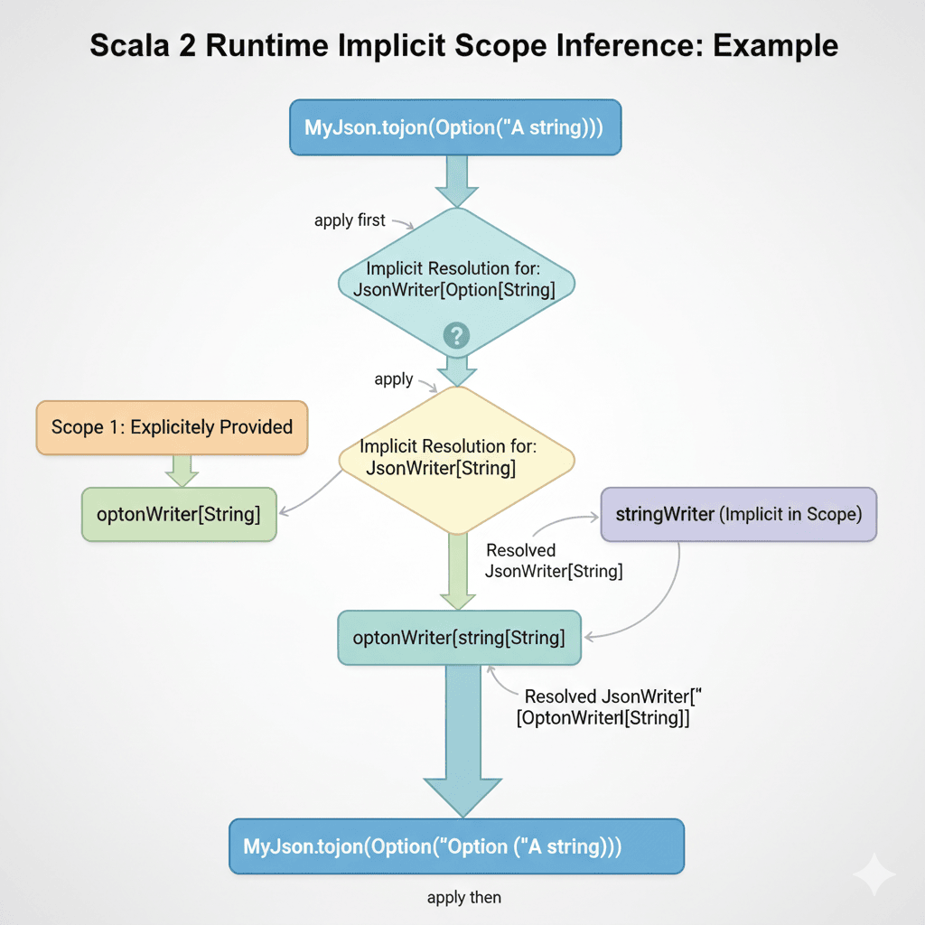
MyJson.toJson(Option("A string"))(optonWriter[String]) // apply first
                                         ⬇️
MyJson.toJson(Option("A string"))(optonWriter(stringWriter)) // apply then

implicit methods with non‐implicit parameters form a different Scala pattern called an implicit conversion, which is an old programming concept.

Key Benefits

• Decoupling: Your data definitions (like case class Person) are separate from their behaviors (like Show).
• Extensibility: You can add Show support for java.util.Date or any other library class without changing its code.
• No Inheritance Tax: You don’t need to make all your classes extend a common Showable trait, which avoids brittle inheritance hierarchies.
• Type-Safe: The compiler guarantees at compile time that the behavior exists for the type you’re using.

(Note: Scala 3 heavily refines this pattern, making it a first-class language feature with given and using clauses, which replace implicits.)

1. Functional Programming in Scala, Ch. 1: “What is functional programming?” → “The benefits of FP: a simple example”, p. 3-12 ↩ ↩² ↩³

2. Category Theory, Ch. 9: “Functors and Natural Transformations” → p. 156-161 ↩

3. Bird & Wadler: Introduction to Functional Programming, Ch. 3: “Lists” → “Map and filter”, p. 61-65 ↩ ↩² ↩³

4. Programming in Scala Fourth Edition, Ch. 23: “For Expressions Revisited” → p. 528-545 ↩

5. Scala in Depth, Ch. 11: “Patterns in functional programming” → “Currying and applicative style”, p. 266-268 ↩ ↩² ↩³

6. Scala with Cats, Ch. 1: “Introduction”, p. 10 -11 ↩