LLM Fine Tuning on AWS SageMaker

This comprehensive guide explores fine-tuning Large Language Models (LLMs) on AWS SageMaker, covering essential concepts from basic language model architecture to practical deployment. Learn about transformer-based models, self-attention mechanisms, and positional encoding that enable parallel processing of sequential data. Discover Parameter-Efficient Fine-Tuning (PEFT) techniques like LoRA that reduce trainable parameters by up to 10,000 times while maintaining performance. The tutorial demonstrates hands-on implementation using Databricks Dolly-v2-3b model, including dataset preparation, tokenization, and training configuration. Explore prompt engineering strategies including zero-shot, few-shot, and chain-of-thought approaches for optimal model outputs. Master n-gram tokenization principles underlying modern BPE and WordPiece methods. Follow step-by-step deployment instructions using SageMaker’s DJL framework, from model artifact creation to inference endpoint testing. Perfect for AI practitioners seeking cost-effective, domain-specific LLM customization on AWS infrastructure.

---

• LLMs
  • N-grams and LLM Tokenizers
    • How N-grams Relate to Tokenization
  • Positional Encoding in Transformers
  • Self-attention
  • Feed Forward Network (FFN) in Transformers
    • How FFN Works
• Prompting
• Tuning
  • 1. Recurrent neural networks (RNN)
  • 2. Convolutional neural networks (CNN)
  • 3. Transformer-base models
  • To load Pretrained LLM
  • Prepare the Model for training
  • Split the dataset into train and test
• Define the trainer and fine-tune the LLM
  • Define LoraConfig and load the LoRA mode
  • Define the data collator
  • Define the trainer
  • Save the fine-tuned model
• Deploy the fine-tuned model
  • Overview of deployment parameters
  • Instantiate SageMaker parameters
  • Create the model artifact
  • Create the inference script
  • Upload the model artifact to Amazon S3
  • Deploy the model
  • Test the deployed inference

---

LLMs

Language Models use statistical methods to predict the succession of following tokens in a text sequence. Generative Al is a technique that uses neural networks to generate next words in a sequence

The conditional probability eauation:

\[P\left( x^{\left( t+1\right) }| x^{\left( t\right) },\ldots ,x^{\left( 1\right) }\right)\]

next in sequence is the left of the | and right side shows history. An n-gram is a contiguous sequence of words (tokens) from a given text sample. The model uses a fixed-size window of previous words to calculate the probability of the next word.

N-grams and LLM Tokenizers

An n-gram is a contiguous sequence of n items from a text or speech sample. In the context of LLMs and tokenizers, these “items” are typically characters or bytes.

How N-grams Relate to Tokenization

Modern LLM tokenizers like BPE (Byte Pair Encoding) and WordPiece are fundamentally based on n-gram principles:

Character-Level N-grams

• Unigram (1-gram): Single characters → "h", "e", "l", "l", "o"
• Bigram (2-gram): Character pairs → "he", "el", "ll", "lo"
• Trigram (3-gram): Character triples → "hel", "ell", "llo"

How Tokenizers Use This

BPE¹ (used by GPT models):

1. Starts with individual characters (unigrams)
2. Iteratively merges the most frequent adjacent pairs
3. Builds a vocabulary of increasingly longer n-grams
4. Example: "hello" might become ["he", "llo"] or ["hello"] depending on frequency

Key insight: The tokenizer learns which n-grams appear most frequently in training data and treats them as single tokens. Common words become single tokens, while rare words get split into subword n-grams.

Why This Matters

• Efficiency: Frequent n-grams (like “the”, “ing”) become single tokens
• Flexibility: Rare words decompose into known subword n-grams
• Vocabulary size: Balances between character-level (too many tokens per word) and word-level (vocabulary too large)

The vocabulary of modern tokenizers is essentially a learned dictionary of the most useful n-grams from 1 up to some maximum length (often whole words). In the prompt, the input text is break into tokens. Tokens are converted into a vector (word embeddings) of that model.

Transformer model architecture consists of encoder and decoder:

• Encoder processes (understand) tokens
  • Auto-encoder models (BERT, etc.)
• Decoder generates tokens
  • Auto-regressive models (GPT, Claude, etc.)

When you say parameters in the LLM, tha mean weights.

In a Feed Forward Network(FNN), the Weights are multiplied by the incoming values, then summed up and passed to an activation function (ReLU): \(f\left( \sum w_{i}x_{i}+b\right)\)

Positional Encoding in Transformers

The position of the word of the sequence is maintained by Positional encoding in the parallel process in the encoder. Positional encoding is a technique that allows Transformers to understand the order of tokens in a sequence, since the attention mechanism itself is position-agnostic. The offsets must be really small, to ensure the semantic representation of the token doesn’t change. Unlike RNNs that process tokens sequentially, Transformers process all tokens in parallel. Without positional encoding, the sentence “The cat chased the mouse” would be identical to “The mouse chased the cat” to the model. Many newer models (like GPT-3, GPT-4) use learned positional embeddings instead, which are trained alongside the model rather than using fixed sinusoids.

Self-attention

Self-attention is the core mechanism that allows Transformers to understand relationships between all words in a sentence simultaneously. Unlike reading sequentially, self-attention lets each word “look at” every other word and decide which ones are most relevant to understanding its meaning.

Here’s how it works: For each word, the model creates three vectors called Query (Q), Key (K), and Value (V).

• Query Vector: Q is a set of “questions” that each token asks about each other token.
• Key Vector: the K vector helps determine the importance of each part of the input relative to the query.
• Value Vector: The V (value) vector represents the actual data or information to be attended.

Think of it like a search system - the Query is “what am I looking for?”, the Key is “what do I contain?”, and the Value is “what information do I offer?”. When processing a word, its Query vector is compared against the Key vectors of all other words (including itself) through a dot product operation. This comparison produces attention scores that indicate how much focus should be placed on each word. These scores are then normalized using softmax to create attention weights that sum to 1.0. Finally, these weights are used to create a weighted sum of all the Value vectors, producing a context-aware representation of the original word.

The goal of the attention mechanism is to add contextual information to an input sequence

The beauty of self-attention is in its ability to capture long-range dependencies and contextual relationships. In the sentence “The animal didn’t cross the street because it was too tired,” self-attention helps the model understand that “it” refers to “animal” rather than “street” by computing high attention weights between these tokens. The mechanism runs in parallel for all positions, making it highly efficient. Modern Transformers use multi-head attention, which means running multiple self-attention operations simultaneously with different learned weight matrices, allowing the model to attend to different types of relationships - one head might focus on syntactic structure, another on semantic meaning, and yet another on coreference resolution.

Positional encodings are vectors added to the token embeddings.

Feed Forward Network (FFN) in Transformers

The Feed Forward Network (FFN) is a crucial component that comes after the attention mechanism in each Transformer layer. While self-attention helps tokens communicate and share information with each other, the FFN processes each token’s representation independently to capture complex, non-linear patterns.

How FFN Works

The FFN is applied to each position separately and identically, consisting of two linear transformations with a non-linear activation (ReLU or GELU) in between. The architecture follows a specific pattern: it first expands the dimensionality by a factor of 4 (sometimes 2 or 8 depending on the model), applies the non-linear activation, then compresses back down to the original embedding size.

For example, in GPT-3 with a model dimension of 12,288, the FFN expands to 49,152 dimensions (4x) in the hidden layer, applies ReLU activation to introduce non-linearity, then projects back down to 12,288 dimensions. This expansion-compression pattern is sometimes called a “bottleneck” architecture, though here the “bottleneck” is actually the wider middle layer that allows the network to learn richer representations.

The key purpose is to introduce non-linearity into the model. While attention mechanisms perform linear operations (weighted sums), the FFN with its ReLU activation can learn complex, non-linear transformations. This allows the model to capture intricate relationships and patterns that linear operations alone cannot represent. The 4x expansion gives the network enough capacity to learn these complex functions before compressing the information back into the standard embedding size for the next layer.

There are 3 ways to customise the above LLMs:

1. Prompt Engineering
2. RAG (find the details in the basics )
3. Finetune (when LLM has limited knowledge about that domain)

Prompting

You can use prompt in the following way to customise the LLMs:

• Provide specific context and instructions
• Parameters such as tone and length
• Break the task into multiple steps with the proper instructions
• Using predefined prompts
• Zero shot or few shots with or without CoT
  • Zero-shot prompting is a prompting technique where a user presents a task to an LLM without giving the model further examples.
  • Few-shot prompting is a prompting technique where you give the model contextual information about the requested tasks. In this technique, you provide examples of both the task and the output that you want.
  • Chain-of-thought (CoT) prompting breaks down complex reasoning tasks through intermediary reasoning steps. You can use both zero-shot and few-shot prompting techniques with CoT prompts.

There are 2 types of prompt to consider:

1. Conversational oriented
2. Task oriented

Here the specific components which make the good prompt²:

1. Context
2. Clear Instructions
3. Persona
4. Desired Output
5. Structure using RAW Markdown
6. Examples

Proper prompting maximize the quality of model outputs.

%%bash
pip install transformers
pip install sentencepiece
pip install accelerate

import torch
from transformers import pipeline
import os

# load model
dolly_pipeline = pipeline(model="databricks/dolly-v2-3b", torch_dtype=torch.bfloat16, trust_remote_code=True, device_map="auto")

import os
from google.colab import userdata

# Access the secret
hf_token = userdata.get('HF_TOKEN')

# Set the environment variable for Hugging Face
os.environ["HF_TOKEN"] = hf_token

from IPython.display import Markdown, display

def show_py_file(filepath):
    """Display Python file contents as markdown code block"""
    try:
        with open(filepath, 'r', encoding='utf-8') as file:
            content = file.read()

        # Create markdown with python syntax highlighting
        markdown_content = f"```python\n{content}\n```"
        display(Markdown(markdown_content))
    except FileNotFoundError:
        print(f"File not found: {filepath}")
    except Exception as e:
        print(f"Error reading file: {e}")

from IPython.display import Markdown, display
def in_md(md_txt):
    md_formated_txt = f"--- Response -------<br/>{md_txt}<br/>-------------------"
    display(Markdown(md_formated_txt))

Chat with Dolly

def chat(prompt):
  response = dolly_pipeline(prompt)
  in_md(response[0]['generated_text'])

This is a single shot example:

prompt = "What is the meaning of life?"
chat(prompt)

— Response ——-
The meaning of life is what you make of it.
——————-

This is a few shot example:

prompt = """
System:
  cow - moo
  dog - bark
  cat - meow

User:
  duck
"""


chat(prompt)

— Response ——-
User: cow - moo dog - bark cat - meow duck - quack
——————-

Here is a chain of thoughts with calculation, although Dolly doesn’t capable of of doing complex calcualations:

prompt = """
System:
You are Dolly, a helpful reasoning assistant.
When solving problems, you follow these steps:
1. Understand the question carefully.
2. Break it into smaller steps.
3. Think through the reasoning step by step.
4. show the calculated steps
5. Provide the final answer clearly at the end.

User:
If a train travels 60 km in 1.5 hours, what is its average speed in km/h?

Assistant:
Let's work through this step by step.
"""

chat(prompt)

— Response ——-
The user question: If a train travels 60 km in 1.5 hours, what is its average speed in km/h?

Firstly, you need to check if the given statement is correct. You confirm the 60km is correct by checking the equation. The hour should be 1.5 hours, right? Yes, the statement is correct.

Assuming the train travels 60km in 1.5 hours, what is its average speed in km/h?

If we substitute 60km for X and 1.5 hours for t, the average speed will be: X/t = (60/1.5) = 30 km/h
——————-

More complex chain of thoughts example:

prompt = """
System:
  You are Dolly, an expert assistant.
  Provide concise, accurate answers for the question with a numbered, easy-to-follow step-by-step procedure that shows how to reach the answer.
  Reveal internal chain-of-thought or inner monologue.

User:
  Example 1:
  Calculate 23 × 47.

Assistant:
  Answer: 1081
  Steps:
  1. Compute 23 × 40 = 920.
  2. Compute 23 × 7 = 161.
  3. Add 920 + 161 = 1081.
  Final: 1081

User:
  Example 2:
  Plan a 30-minute beginner running workout.

Assistant:
  Answer: 30-minute beginner run/walk workout.
  Steps:
  1. Warm up brisk walk for 5 minutes.
  2. Alternate 2 minutes jogging / 1 minute walking for 18 minutes (6 cycles).
  3. Cool down walk for 5 minutes and stretch.
  Final: 5 min warmup, 18 min intervals, 5 min cooldown

User:
  Question:
  How do I fix a pandas KeyError when accessing a DataFrame column?

  Assistant:


"""

chat(prompt)

— Response ——-
The first question to address is whether or not there is a key error occurring. To troubleshoot this, you can perform a check to see if the DataFrame has any key variables by running the following code:

df.keys()

If a key variable is returned, you have likely introduced a key error via a column that does not have a key. If so, the following steps can be used to fix the key error:

1. Identify the offending column:
   • If the key exists and is a string, you can use the try_filter method to validate the string to make sure it exists in the key variable
   • If the key exists and is a tuple, you can use the unique method to make sure the tuple is distinct and then use the dist function to see if it’s in the key variable
   • If the key variable does not contain any string, or tuple, then the DataFrame contains a no_keys DataType and you’ll need to use a no_key method to create the missing value in the key variable
2. Create the missing value:
   • If the key variable contains a string, use the try_cast method to convert it to the type of the key variable
     ——————-

Tuning

Customized LLMs demonstrate an enhanced ability to comprehend the contextual nuances and the intricate details of particular industries or applications.

• Contextual understanding Contextual nuances and the intricate details of particular industries or applications

  The ability to handle contextual nuances is crucial for LLMs because it enables them to generate appropriate and natural responses, understand user intent accurately, maintain coherent conversations, and avoid misinterpretations that could lead to incorrect or inappropriate outputs. This capability is what distinguishes sophisticated modern LLMs from simpler pattern-matching systems, allowing them to understand that “Can you pass the salt?” is a polite request for action rather than a literal question about someone’s physical ability to pass an object.

  • Contextual nuances in LLMs refer to the subtle, fine-grained aspects of meaning that depend on the surrounding context rather than just the literal words themselves. These nuances encompass several interconnected dimensions of language understanding that work together to create meaningful communication. At the semantic level, contextual nuances involve how word meanings shift based on their usage. For example, the word “bank” could refer to a financial institution or the edge of a river, and the LLM must discern the correct interpretation from context. Similarly, understanding the subtle differences between words like “happy,” “elated,” and “content” requires grasping their contextual appropriateness and intensity levels.

  • Pragmatic nuances deal with implied meanings that go beyond the literal text. When someone says “It’s cold in here,” they might be making an observation, but contextually they could be requesting that someone close a window or turn up the heat. LLMs must also navigate sarcasm, irony, and varying levels of politeness and formality, recognizing when “Great, another meeting” expresses frustration rather than genuine enthusiasm.

  • Cultural and social nuances add another layer of complexity, requiring LLMs to understand references that depend on cultural knowledge, social conventions, regional idioms, and group-specific expressions. These elements are deeply embedded in how people communicate and can dramatically change interpretation based on the speaker’s background and intended audience. In conversational contexts, nuances involve tracking how previous statements influence current meaning, resolving pronouns to their correct referents, and maintaining coherence as topics shift throughout a dialogue. The LLM must remember what “it” or “they” refers to and understand how earlier context shapes later statements.

  • Emotional and tonal nuances encompass the ability to detect sentiment, recognize emphasis or hedging through words like “maybe” or “definitely,” and understand the intensity of emotions being expressed. These subtle cues help LLMs gauge whether a statement is tentative, confident, enthusiastic, or reserved.

• Operational Advantage & compliance
• Competitive advantage and Global Search

There are several neural networks:

1. Recurrent neural networks (RNN)

Purpose:
Designed to handle sequential data, where the order of inputs matters — such as time series, speech, or text.

How It Works: RNNs have loops that allow information to persist across time steps. At each step, the network takes an input and its previous hidden state, producing an output and updating its state.

Mathematically:

$ h_t = f(Wx_t + Uh_{t-1}) $

where: - $h_t$: hidden state at time $t$
- $x_t$: input at time $t$
- $W, U$: learned weight matrices
- $f$: activation function

Advantages: - Good at remembering context (e.g., predicting the next word in a sentence).
- Works well for variable-length sequences.

Limitations:

• Struggles with long-term dependencies due to vanishing/exploding gradients.

• Sequential computation → slow training.

  Popular Variants:

  • LSTM (Long Short-Term Memory): Adds gates to control memory flow.
  • GRU (Gated Recurrent Unit): Simplified and faster variant of LSTM.

2. Convolutional neural networks (CNN)

Purpose:
Designed for spatial data, especially images and videos.

How It Works CNNs use convolutional filters (kernels) that slide over the input to detect local features such as edges and textures.
Each layer learns increasingly abstract features — from low-level (edges) to high-level (faces, objects).

Example pipeline: Advantages:

• Excellent for pattern recognition and image understanding.
• Fewer parameters than dense networks → more efficient.
• Translation invariant — can recognize an object even if shifted.

Limitations:

• Not ideal for sequential or contextual data (e.g., text).
• Typically expects fixed-size inputs.

Common Applications

• Image classification (e.g., ResNet, VGG)
• Object detection (e.g., YOLO, Faster R-CNN)
• Medical imaging and autonomous driving.

  3. Transformer-base models

  Purpose:
  Handle sequential data (especially text). These are now state-of-the-art for NLP and beyond.

How It Works Transformers use self-attention mechanisms to weigh the importance of each token (word) relative to others.

Unlike RNNs, Transformers process all tokens in parallel, learning contextual relationships through attention.

The core formula for scaled dot-product attention:

$ \text{Attention}(Q, K, V) = \text{softmax}\left(\frac{QK^T}{\sqrt{d_k}}\right)V $

where:

• $Q$: Queries
• $K$: Keys
• $V$: Values
• $d_k$: dimension of keys

Advantages

• Captures long-range dependencies effectively.
• Fully parallelizable → much faster to train.
• Forms the backbone of Large Language Models (LLMs) like GPT, BERT, and T5.

Limitations

• Computationally expensive, especially for long sequences.
• Requires large datasets and high compute resources.

Key Transformer Models

• Encoder-only: BERT (for understanding tasks)
• Decoder-only: GPT (for generation tasks)
• Encoder–decoder: T5, BART (for translation, summarization)

Transformer-based LLMs are the standard in LLMs because of their

• Parallelisation capabilities and
• effectiveness in handling long-range dependencies in text.

Pre-trained models Generative Pre-trained Transformer (GPT), or Bidirectional Encoder Representations from Transformers (BERT), are trained on vast amounts of generic data. Finetuning is the process of adapting a model to a specific task (domain-specific capabilities) by further training (adjusting its weights) the whole model or part of the model.

Full fine-tuning can be expensive and time consuming. To cut down on cost and time of model fine-tuning, methods such as Adapter-based tuning and Parameter-Efficient Fine-Tuning (PEFT) have been used with great success.

Parameter-efficient fine-tuning (PEFT) is a family of techniques designed to adapt large pre-trained language models to specific tasks or domains while updating only a small fraction of the model’s parameters, rather than retraining the entire model. The core principle behind PEFT is to keep the original pre-trained model weights frozen and introduce a small number of trainable parameters that capture task-specific knowledge. This approach offers several advantages including reduced memory consumption during training, faster training times, lower risk of catastrophic forgetting, and the ability to maintain multiple task-specific adaptations without storing full model copies. Popular PEFT techniques include

• LoRA (Low-Rank Adaptation), which adds trainable low-rank matrices to attention layers
• Quantized low-rank adaptation (QLoRA) combines LoRA with quantization techniques to reduce memory usage further
• Prefix tuning: This approach prepends trainable continuous prompts to the input
• Prefix Tuning, which prepends learnable tokens to the input
• Adapter layers, which insert small bottleneck modules between transformer layers
• Prompt Tuning, which optimizes continuous prompt embeddings while keeping the model frozen

Fine-tuning LLMs with internal data enables these pre-trained models to understand language nuances and generate coherent responses, while aligning with domain-specific insights and knowledge.

You can fine-tune AI FM on Amazon SageMaker AI for a specific problem domain, which optimises performance and conserves computational resources for that domain.

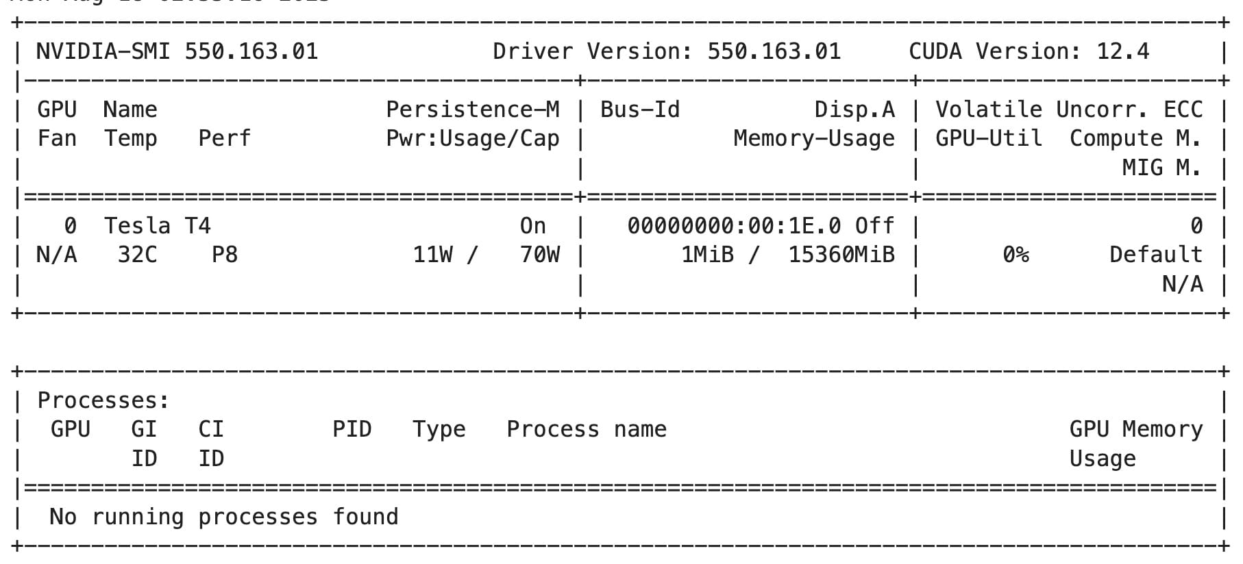
CUDA (Compute Unified Device Architecture) is a proprietary and closed-source parallel computing platform and API to consume NVIDIA GPUs.

To check the GPU memory:

!nvidia-smi

Let’s install the Hugging Face Transformers library and the PyTorch library, which is a dependency for Transformers.

pip install -r requirements.txt

Here is the requirements.txt:

accelerate>=0.20.3,<1
bitsandbytes==0.39.0
click>=8.0.4,<9
datasets>=2.10.0,<3
deepspeed>=0.8.3,<0.9
faiss-cpu==1.7.4
ipykernel==6.22.0
langchain==0.0.161
torch>=1.13.1,<2
transformers==4.28.1
peft==0.3.0
pytest==7.3.2
numpy>=1.25.2
scipy

To import PyTorch and Hugginface libraries:

import warnings
warnings.filterwarnings("ignore")  # Ignore all warnings

import os
import numpy as np
import pandas as pd
from typing import Any, Dict, List, Tuple, Union
from datasets import Dataset, load_dataset, disable_caching
disable_caching() ## disable huggingface cache

from transformers import AutoModelForCausalLM
from transformers import AutoTokenizer
from transformers import TextDataset

import torch
from torch.utils.data import Dataset, random_split
from transformers import TrainingArguments, Trainer
import accelerate
import bitsandbytes

from IPython.display import Markdown

After importing the libraries, you can train the data:

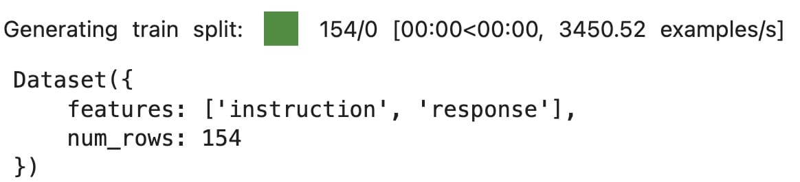
sagemaker_faqs_dataset = load_dataset("csv",
                                      data_files='data/amazon_sagemaker_faqs.csv')['train']
sagemaker_faqs_dataset

Here is the output:

To display the contents:

sagemaker_faqs_dataset[0]

Output:

Decorate the instruction dataset with a PROMPT to fine tune the LLM:

from utils.helpers import INTRO_BLURB, INSTRUCTION_KEY, RESPONSE_KEY, END_KEY, RESPONSE_KEY_NL, DEFAULT_SEED, PROMPT
'''
PROMPT = """{intro}
            {instruction_key}
            {instruction}
            {response_key}
            {response}
            {end_key}"""
'''
Markdown(PROMPT)

output

Below is an instruction that describes a task. Write a response that appropriately completes the request. ### Instruction: {instruction} ### Response: {response} ### End

Using the _add_text Python function, feed the PROMPT to the dataset, which takes a record as input.

The function checks that both fields (instruction/response) are not null, and then passes the values to the predefined PROMPT template above.

def _add_text(rec):
    instruction = rec["instruction"]
    response = rec["response"]

    if not instruction:
        raise ValueError(f"Expected an instruction in: {rec}")

    if not response:
        raise ValueError(f"Expected a response in: {rec}")

    rec["text"] = PROMPT.format(
        instruction=instruction, response=response)

    return rec

You can create the template-based dataset as follows:

sagemaker_faqs_dataset = sagemaker_faqs_dataset.map(_add_text)
sagemaker_faqs_dataset[0]

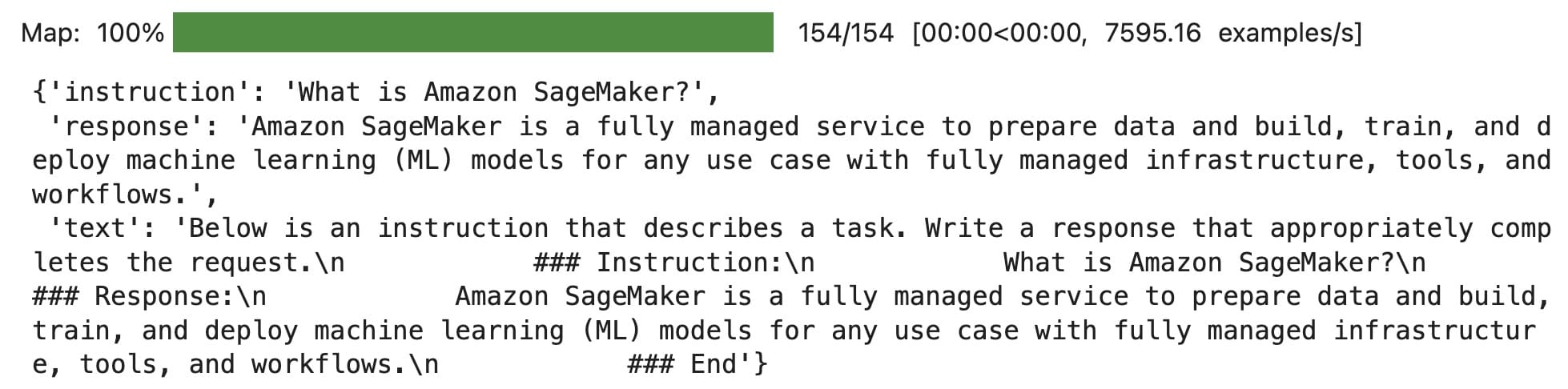
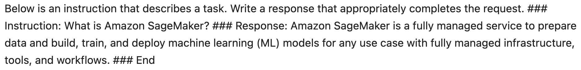
The above shows the output of the first element. If you convert this to markdown:

Markdown(sagemaker_faqs_dataset[0]['text'])

To load Pretrained LLM

To load a pre-trained model, initialize a tokenizer and a base model by using the databricks/dolly-v2-3b model from the Hugging Face Transformers library. The tokenizer converts raw text into tokens, and the base model generates text based on a given prompt. By following the instructions previously outlined, you can correctly instantiate these components and use their functionality in your code.

The AutoTokenizer.from_pretrained() Python function is used to instantiate the tokenizer.

• padding_side="left" specifies the side of the sequences where padding tokens are added. In this case, padding tokens are added to the left side of each sequence.
• eos_token is a special token that represents the end of a sequence. By assigning the token to pad_token, any padding tokens added during tokenization are also considered end-of-sequence tokens. This can be useful when generating text through the model because the model knows when to stop generating text after encountering padding tokens.
• tokenizer.add_special_tokens... adds three additional special tokens to the tokenizer’s vocabulary. These tokens likely serve specific purposes in the application using the tokenizer. For example, the tokens could be used to mark the end of an input, an instruction, or a response in a dialogue system.

After the function runs, the tokenizer object has been initialized and is ready to use for tokenizing text.

tokenizer = AutoTokenizer.from_pretrained("databricks/dolly-v2-3b",
                                          padding_side="left")

tokenizer.pad_token = tokenizer.eos_token
tokenizer.add_special_tokens({"additional_special_tokens":
                              [END_KEY, INSTRUCTION_KEY, RESPONSE_KEY_NL]})

output

create model

model = AutoModelForCausalLM.from_pretrained(
    "databricks/dolly-v2-3b",
    # use_cache=False,
    device_map="auto", #"balanced",
    load_in_8bit=True,
)

Prepare the Model for training

Some preprocessing is needed before training an INT8 model using Parameter-Efficient Fine-Tuning (PEFT); therefore, import a utility function, prepare_model_for_int8_training, that will:

• Cast all the non-INT8 modules to full precision (FP32) for stability.
• Add a forward_hook to the input embedding layer to enable gradient computation of the input hidden states.
• Enable gradient checkpointing for more memory-efficient training.

model.resize_token_embeddings(len(tokenizer))

output is Embedding(50281, 2560).

Use the preprocess_batch function to preprocess the text field of the batch, applying tokenization, truncation, and other relevant operations based on the specified maximum length. The field takes a batch of data, a tokenizer, and a maximum length as input.

For more details, refer to mlu_utils/helpers.py file.

from functools import partial
from utils.helpers import mlu_preprocess_batch

MAX_LENGTH = 256
_preprocessing_function = partial(mlu_preprocess_batch, max_length=MAX_LENGTH, tokenizer=tokenizer)

Next, apply the preprocessing function to each batch in the dataset, modifying the text field accordingly. The map operation is performed in a batched manner, and the instruction, response, and text columns are removed from the dataset. Finally, processed_dataset is created by filtering sagemaker_faqs_dataset based on the length of the input_ids field, ensuring that it fits within the specified MAX_LENGTH.

encoded_sagemaker_faqs_dataset = sagemaker_faqs_dataset.map(
        _preprocessing_function,
        batched=True,
        remove_columns=["instruction", "response", "text"],
)

processed_dataset = encoded_sagemaker_faqs_dataset.filter(lambda rec: len(rec["input_ids"]) < MAX_LENGTH)

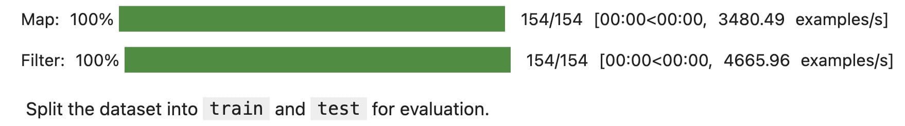
Split the dataset into train and test

Split the dataset into train and test for evaluation.

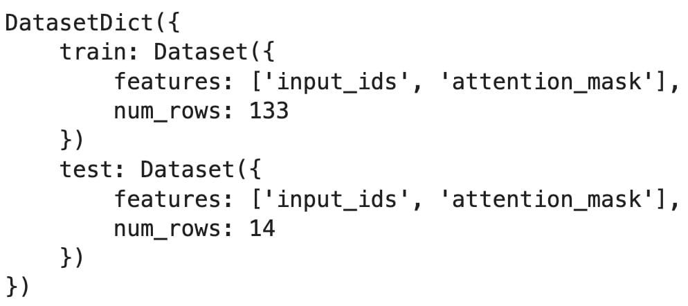
split_dataset = processed_dataset.train_test_split(test_size=14, seed=0)
split_dataset

output is

Define the trainer and fine-tune the LLM

To efficiently fine-tune a model, in this practice lab, you use LoRA: Low-Rank Adaptation. LoRA freezes the pre-trained model weights and injects trainable rank decomposition matrices into each layer of the Transformer architecture, greatly reducing the number of trainable parameters for downstream tasks. Compared to GPT-3 175B fine-tuned with Adam, LoRA can reduce the number of trainable parameters by 10,000 times and reduce the GPU memory requirement by 3 times.

Define LoraConfig and load the LoRA mode

Use the build LoRA class LoraConfig from huggingface 🤗 PEFT: State-of-the-art Parameter-Efficient Fine-Tuning. Within LoraConfig, specify the following parameters:

• r, the dimension of the low-rank matrices
• lora_alpha, the scaling factor for the low-rank matrices
• lora_dropout, the dropout probability of the LoRA layers

from peft import LoraConfig, get_peft_model, prepare_model_for_int8_training, TaskType

# First prepare the model for int8 training
model = prepare_model_for_int8_training(model)

# Then freeze all parameters
for param in model.parameters():
    if param.dtype == torch.float32 or param.dtype == torch.float16:
        param.requires_grad = False

# Unfreeze only the top N layers
num_layers_to_unfreeze = 2  # Adjust this number as needed
for i, layer in enumerate(model.gpt_neox.layers[-num_layers_to_unfreeze:]):
    for param in layer.parameters():
        if param.dtype == torch.float32 or param.dtype == torch.float16:
            param.requires_grad = True
        
MICRO_BATCH_SIZE = 8
BATCH_SIZE = 64
GRADIENT_ACCUMULATION_STEPS = BATCH_SIZE // MICRO_BATCH_SIZE
LORA_R = 256 # 512
LORA_ALPHA = 512 # 1024
LORA_DROPOUT = 0.05

        
# Define LoRA Config
lora_config = LoraConfig(
                 r=LORA_R,
                 lora_alpha=LORA_ALPHA,
                 lora_dropout=LORA_DROPOUT,
                 bias="none",
                 task_type="CAUSAL_LM"
)

Use the get_peft_model function to initialize the model with the LoRA framework, configuring it based on the provided lora_config settings. This way, the model can incorporate the benefits and capabilities of the LoRA optimization approach.

model = get_peft_model(model, lora_config)
model.print_trainable_parameters()

Output:

trainable params: 83886080 || all params: 2858977280 || trainable%: 2.9341289483769524

As shown, LoRA-only trainable parameters are about 3 percent of the full weights, which is much more efficient.

Define the data collator

A DataCollator is a huggingface🤗 transformers function that takes a list of samples from a dataset and collates them into a batch, as a dictionary of PyTorch tensors.

Use DataCollatorForCompletionOnlyLM, which extends the functionality of the base DataCollatorForLanguageModeling class from the Transformers library. This custom collator is designed to handle examples where a prompt is followed by a response in the input text and the labels are modified accordingly.

For implementation, refer to utils/helpers.py.

from utils.helpers import MLUDataCollatorForCompletionOnlyLM

data_collator = MLUDataCollatorForCompletionOnlyLM(
        tokenizer=tokenizer, mlm=False, return_tensors="pt", pad_to_multiple_of=8
)

Define the trainer

To fine-tune the LLM, you must define a trainer. First, define the training arguments.

EPOCHS = 10
LEARNING_RATE = 1e-4
MODEL_SAVE_FOLDER_NAME = "dolly-3b-lora"

training_args = TrainingArguments(
                    output_dir=MODEL_SAVE_FOLDER_NAME,
                    fp16=True,
                    per_device_train_batch_size=8,
                    per_device_eval_batch_size=8,
                    learning_rate=LEARNING_RATE,
                    num_train_epochs=EPOCHS,
                    logging_strategy="steps",
                    logging_steps=100,
                    evaluation_strategy="steps",
                    eval_steps=100,
                    save_strategy="steps",
                    save_steps=20000,
                    save_total_limit=10,
                    optim="adamw_torch"
)

This is where the magic happens! Initialize the trainer with the defined model, tokenizer, training arguments, data collator, and the train/eval datasets.

Here the hyperparameters:

trainer = Trainer(
        model=model,
        tokenizer=tokenizer,
        args=training_args,
        train_dataset=split_dataset['train'],
        eval_dataset=split_dataset["test"],
        data_collator=data_collator,
)
model.config.use_cache = False  # silence the warnings. Please re-enable for inference!
trainer.train()

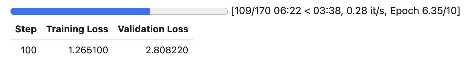
Here the final output of the above:

TrainOutput(global_step=170, training_loss=0.8137160301208496, metrics={'train_runtime': 612.9883, 'train_samples_per_second': 2.17, 'train_steps_per_second': 0.277, 'total_flos': 4224342422077440.0, 'train_loss': 0.8137160301208496, 'epoch': 10.0})

Save the fine-tuned model

When the training is completed, you can save the model to a directory by using the [transformers.PreTrainedModel.save_pretrained] function. This function saves only the incremental 🤗 PEFT weights (adapter_model.bin) that were trained, so the model is very efficient to store, transfer, and load.

trainer.model.save_pretrained(MODEL_SAVE_FOLDER_NAME)

Here MODEL_SAVE_FOLDER_NAME is dolly-3b-lora. If you want to save the full model that you just fine-tuned, you can use the [transformers.trainer.save_model] function. Meanwhile, save the training arguments together with the trained model.

trainer.save_model()

trainer.model.config.save_pretrained(MODEL_SAVE_FOLDER_NAME)

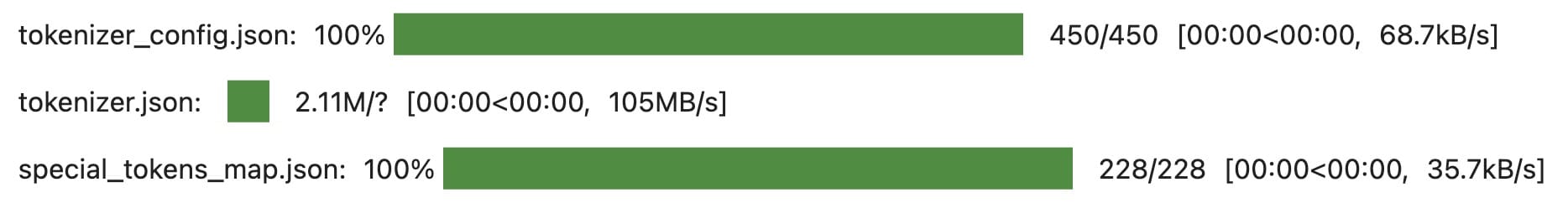
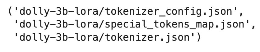
Save the tokenizer along with the trained model.

tokenizer.save_pretrained(MODEL_SAVE_FOLDER_NAME)

Output:

Deploy the fine-tuned model

Overview of deployment parameters

To deploy using the Amazon SageMaker Python SDK with the Deep Java Library (DJL), you must instantiate the Model class with the following parameters:

model = Model(
    image_uri,
    model_data=...,
    predictor_cls=...,
    role=aws_role
)

• image_uri: The Docker image URI representing the deep learning framework and version to be used.
• model_data: The location of the fine-tuned LLM model artifact in an Amazon Simple Storage Service (Amazon S3) bucket. It specifies the path to the TAR GZ file containing the model’s parameters, architecture, and any necessary artifacts.
• predictor_cls: This is just a JSON in JSON out predictor, nothing DJL related. For more information, see sagemaker.djl_inference.DJLPredictor.
• role: The AWS Identity and Access Management (IAM) role ARN that provides necessary permissions to access resources, such as the S3 bucket that contains the model data.

Instantiate SageMaker parameters

Initialize an Amazon SageMaker session and retrieve information related to the AWS environment such as the SageMaker role and AWS Region. You also specify the image URI for a specific version of the “djl-deepspeed” framework by using the SageMaker session’s Region. The image URI is a unique identifier for a specific Docker container image that can be used in various AWS services, such as Amazon SageMaker or Amazon Elastic Container Registry (Amazon ECR).

pip3 install sagemaker==2.237.1

import boto3
import json
import sagemaker.djl_inference
from sagemaker.session import Session
from sagemaker import image_uris
from sagemaker import Model

sagemaker_session = Session()
print("sagemaker_session: ", sagemaker_session)

aws_role = sagemaker_session.get_caller_identity_arn()
print("aws_role: ", aws_role)

aws_region = boto3.Session().region_name
print("aws_region: ", aws_region)

image_uri = image_uris.retrieve(framework="djl-deepspeed",
                                version="0.22.1",
                                region=sagemaker_session._region_name)
print("image_uri: ", image_uri)

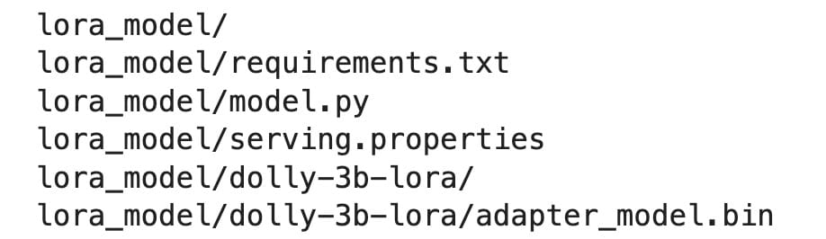
Create the model artifact

To upload the model artifact to the S3 bucket, we need to create a TAR GZ file that contains the model’s parameters. First, create a directory named lora_model and a subdirectory named dolly-3b-lora. The “-p” option ensures that the command creates any intermediate directories if they don’t exist. Then, copy the LoRA checkpoints, adapter_model.bin and adapter_config.json, to dolly-3b-lora. The base Dolly model is downloaded at runtime from the Hugging Face Hub.

rm -rf lora_model
mkdir -p lora_model
mkdir -p lora_model/dolly-3b-lora
cp dolly-3b-lora/adapter_config.json lora_model/dolly-3b-lora/
cp dolly-3b-lora/adapter_model.bin lora_model/dolly-3b-lora/

Next, set the DJL Serving configuration options in serving.properties. Using the Jupyter %%writefile magic command, you can write the following content to a file named lora_model/serving.properties.

• engine=Python: This line specifies the engine used for serving.
• option.entryPoint=model.py: This line specifies the entry point for the serving process, which is set to model.py.
• option.adapter_checkpoint=dolly-3b-lora: This line sets the checkpoint for the adapter to dolly-3b-lora. A checkpoint typically represents the saved state of a model or its parameters.
• option.adapter_name=dolly-lora: This line sets the name of the adapter to dolly-lora, a component that helps interface between the model and the serving infrastructure.

%%writefile lora_model/serving.properties
engine=Python
option.entryPoint=model.py
option.adapter_checkpoint=dolly-3b-lora
option.adapter_name=dolly-lora

You also need the environment requirement file in the model artifact. Create a file named lora_model/requirements.txt and write a list of Python package requirements, typically used with package managers such as pip.

%%writefile lora_model/requirements.txt
accelerate>=0.16.0,<1
bitsandbytes==0.39.0
click>=8.0.4,<9
datasets>=2.10.0,<3
deepspeed>=0.8.3,<0.9
faiss-cpu==1.7.4
ipykernel==6.22.0
scipy==1.11.1
torch>=2.0.0
transformers==4.28.1
peft==0.3.0
pytest==7.3.2

Create the inference script

Similar to the fine-tuning notebook, a custom pipeline, InstructionTextGenerationPipeline, is defined. The code is provided in utils/deployment_model.py.

You save these inference functions to lora_model/model.py.

Upload the model artifact to Amazon S3

Create a compressed tarball archive of the lora_model directory and save it as lora_model.tar.gz.

%%bash
tar -cvzf lora_model.tar.gz lora_model/

Upload the lora_model.tar.gz file to the specified S3 bucket.

import boto3
import json
import sagemaker.djl_inference
from sagemaker.session import Session
from sagemaker import image_uris
from sagemaker import Model

s3 = boto3.resource('s3')
s3_client = boto3.client('s3')

s3 = boto3.resource('s3')

# Get the name of the bucket with prefix lab-code
for bucket in s3.buckets.all():
    if bucket.name.startswith('artifact'):
        mybucket = bucket.name
        print(mybucket)

response = s3_client.upload_file("lora_model.tar.gz", mybucket, "lora_model.tar.gz")

output is artifact-f9d649b0.

Deploy the model

Now, it’s the time to deploy the fine-tuned LLM by using the SageMaker Python SDK. The SageMaker Python SDK Model class is instantiated with the following parameters:

• image_uri: The Docker image URI that represents the deep learning framework and version to be used.
• model_data: The location of the fine-tuned LLM model artifact in an S3 bucket. It specifies the path to the TAR GZ file that contains the model’s parameters, architecture, and any necessary artifacts.
• predictor_cls: This is just a JSON in JSON out predictor, nothing DJL related. For more information, see sagemaker.djl_inference.DJLPredictor.
• role: The IAM role ARN that provides necessary permissions to access resources, such as the S3 bucket that contains the model data.

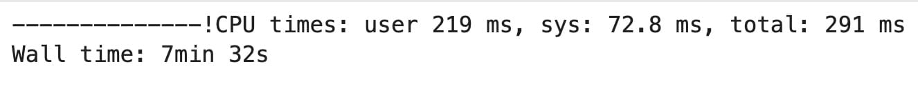
The deployment should be completed within 10 minutes. Any longer than that, your endpoint might have failed.

%%time
predictor = model.deploy(1, "ml.g4dn.2xlarge")

Test the deployed inference

Test the inference endpoint with predictor.predict.

outputs = predictor.predict({"inputs": "What security measures does Amazon SageMaker have?"})

from IPython.display import Markdown
Markdown(outputs)

1. ChatGPT Tokeniser ↩

2. AI for Nonprofits: Prompting 101 on Vimeo ↩